ICIS 2023: Why I love India so much!

In a few hours I’ll be returning to the Great State of Texas from India, where I’ve been attending the ICIS 2023 Conference. I had the opportunity to meet with WarpPLS users, which I always enjoy very much, and with methodological researchers doing PLS-related work.

Talking about people doing PLS-related work, it was a special treat to be able to meet and talk with Nicholas Danks. The man is a true scholar and a genius. I hope to collaborate with him in the future, and (perhaps, if I am lucky) get some of that talent through osmosis.

Another highlight was talking again with the incomparable Dr. Boo. I was busy distracting her with nonsense when her name was mentioned at the awards ceremony. For those of you who don’t know, she is one of the forerunners of the field of Information Systems, a field that she begun influencing at the young age of 13 (according to my calculations).

This was my first time in India. I loved it so much! This was such a nice experience in no small measure due to Glory George, who was kind enough to show me some of Hyderabad. The people of India are so smart and hard working. Take for example the person on the photo below; he solved a 100-year-old numeric computing problem while riding on the back of a bike in heavy traffic!

Okay, just my imagination. But he was indeed doing what seemed to be some coding, using his friend’s constantly moving upper back as a table. By the way, if you think that traffic in India is chaotic, think again. Those who pay close attention will notice that there is method to what looks like disorderly flow. More than method actually, it is a form of art. Just don’t try driving if you are a beginner; it will be like challenging Ma Long to a “ping pong” match.

Should you want to see and hear the person who is writing this, in keeping with media naturalness theory, check this video. More views and likes will help make my dear friends Steve Harmon and Rolando Santos happy about their masterful video creation and editing work.

Best regards to all!

WarpPLS: A bit of history

The YouTube video linked below (scroll down to the end of the news article) provides a bit of history in connection with the development of WarpPLS. A big thank you to Rolando Santos for his professional video creation work!

https://www.tamiu.edu/newsinfo/2023/10/topworldresearcher10262023.shtml

Best regards to all!

Robustness tests in PLS-SEM: Video for the Qatar Chapter of the Decision Sciences Institute

The so-called "robustness" tests that some refer to, in connection with PLS-SEM, are generally tests of: nonlinearity, common method bias, and endogeneity. In WarpPLS, nonlinearity can be tested via full latent growth, commom method bias via FCVIFs, and endogeneity via instrumental variables. The video linked below covers most of these issues.

https://youtu.be/I3YYdpdXhII

This video is of a presentation to faculty and students at the Qatar Chapter of the Decision Sciences Institute on the topics of factor-based PLS-SEM (PLSF-SEM), endogeneity, and common method bias. (SEM = structural equation modeling.) Addressing these issues helps with publishing in top-tier information systems and decision sciences journals, among others.

Best regards to all!

Individual paths can be set as linear or nonlinear in PLS-SEM analyses

In WarpPLS, the “View or change individual inner model analysis algorithm settings” option allows you to set inner model algorithms for individual paths in PLS-SEM analyses; whether these analyses are composite-based or factor-based. That is, for each path a user can select a different algorithm from among the following choices: “Linear”, “Warp2”, “Warp2 Basic”, “Warp3”, and “Warp3 Basic”.

This option is particularly useful in empirical investigations where researchers have solid theoretical reasons to expect certain paths to be associated with nonlinear relationships of particular types. Those researchers may also have solid theoretical reasons to expect certain paths to be associated with linear relationships. Given that one of the main goals of SEM is to test theory, theoretical considerations should be given a very high priority in the selection of algorithms to be used for each path in a model.

There is a short video that illustrates this ().

On a related note - since classic moderating effects analyses already capture nonlinearity, it is usually advisable for users to set moderating paths as linear. They can do this even as they set direct paths as nonlinear. This leads to 2D graphs that are easier to interpret. If users set moderating paths as nonlinear, their interpretation becomes more difficult, as more complex types of moderating relationships are captured.

How to theorize nonlinear relationships and test them: A journal article example

How can a researcher theorize nonlinear relationships and test them? This question is addressed through the publication below, which provides an example of nonlinear theorizing and related empirical analysis. To the best of our knowledge, this is one of the first articles that exemplifies how nonlinear theorizing can be incorporated into a casual model and tested with WarpPLS.

Kock, N., Mayfield, M., Mayfield, J., Sexton, S., & De La Garza, L. (2019). Empathetic leadership: How leader emotional support and understanding influences follower performance. Journal of Leadership and Organizational Studies, 26(2), 217-236.

A link to a PDF file is available ().

Abstract:

This article presents a theory of empathetic leadership and its initial test. Empathetic leadership provides a model of how leader understanding and support improves follower behaviors and affective states. For this article, we explored the link between empathetic leadership and follower performance. Specifically, we tested the causal processes by which empathetic language influences follower performance. These processes include follower job satisfaction and innovation. Findings support model hypotheses and provide preliminary causal support for the model.

Advantages of nonlinear over segmentation analyses in path models

Nonlinear analyses employing the software WarpPLS allow for the identification of linear segments emerging from a nonlinear analysis, but without the need to generate subsamples. A new article is available demonstrating the advantages of nonlinear over data segmentation analyses. These include a larger overall sample size for calculation of P values, and the ability to uncover very high segment-specific path coefficients. Its reference, abstract, and link to full text are available below.

Kock, N. (2016). Advantages of nonlinear over segmentation analyses in path models. International Journal of e-Collaboration, 12(4), 1-6.

The recent availability of software tools for nonlinear path analyses, such as WarpPLS, enables e-collaboration researchers to take nonlinearity into consideration when estimating coefficients of association among linked variables. Nonlinear path analyses can be applied to models with or without latent variables, and provide advantages over data segmentation analyses, including those employing finite mixture segmentation techniques (a.k.a. FIMIX). The latter assume that data can be successfully segmented into subsamples, which are then analyzed with linear algorithms. Nonlinear analyses employing WarpPLS also allow for the identification of linear segments mirroring underlying nonlinear relationships, but without the need to generate subsamples. We demonstrate the advantages of nonlinear over data segmentation analyses.

Among other things this article shows that identification of linear segments emerging from a nonlinear analysis with WarpPLS allows for: (a) a larger overall sample size for calculation of P values, which enables researchers to uncover actual segment-specific effects that could otherwise be rendered non-significant due to a combination of underestimated path coefficients and small subsample sizes; and (b) the ability to uncover very high segment-specific path coefficients, which could otherwise be grossly underestimated.

Enjoy!

Simpson’s paradox, moderation, and the emergence of quadratic relationships in path models

Among the many innovative features of WarpPLS are those that deal with identification of Simpson’s paradox and modeling of nonlinear relationships. A new article discussing various issues that are important for the understanding of the usefulness of these features is now available. Its reference, abstract, and link to full text are available below.

Kock, N., & Gaskins, L. (2016). Simpson’s paradox, moderation, and the emergence of quadratic relationships in path models: An information systems illustration. International Journal of Applied Nonlinear Science, 2(3), 200-234.

While Simpson’s paradox is well-known to statisticians, it seems to have been largely neglected in many applied fields of research, including the field of information systems. This is problematic because of the strange nature of the phenomenon, the wrong conclusions and decisions to which it may lead, and its likely frequency. We discuss Simpson’s paradox and interpret it from the perspective of path models with or without latent variables. We define it mathematically and argue that it arises from incorrect model specification. We also show how models can be correctly specified so that they are free from Simpson’s paradox. In the process of doing so, we show that Simpson’s paradox may be a marker of two types of co-existing relationships that have been attracting increasing interest from information systems researchers, namely moderation and quadratic relationships.

Among other things this article shows that: (a) Simpson’s paradox may be caused by model misspecification, and thus can in some cases be fixed by proper model specification; (b) a type of model misspecification that may cause Simpson’s paradox involves missing a moderation relationship that exists at the population level; (c) Simpson’s paradox may actually be a marker of nonlinear relationships of the quadratic type, which are induced by moderation; and (d) there is a duality involving moderation and quadratic relationships, which requires separate and targeted analyses for their proper understanding.

Enjoy!

Interview video: Conference on Information Systems in Latin America

Recently an interview was conducted for the 3rd Conference on Information Systems in Latin America. In it, Dr. Ned Kock was interviewed by Dr. Alexandre Graeml. The topics covered include: structural equation modeling (SEM), partial least squares (PLS) and related techniques, PLS-based SEM, covariance-based SEM, factors versus composites, nonlinear analyses, and WarpPLS.

WarpPLS and its application to research in business and information systems

The link below is for the Conference’s web site.

ISLA 2016 - Information Systems in Latin America Conference

Enjoy!

Conducting a nonlinear robust path analysis

What if a researcher has only one measure for each latent variable, and still wants to perform a nonlinear “robust” analysis where no parametric assumptions (e.g., univariate or multivariate normality) are made beforehand?

This would call for a new nonlinear robust multivariate analysis approach – a nonlinear robust path analysis. Through this approach the variables in the structural model would not be “latent”, strictly speaking, and thus other assessments would have to be performed in place of a confirmatory factor analysis. That is, without multiple indicators per latent variable measurement, quality assessments must deviate somewhat from what would be used in a traditional structural equation modeling analysis.

An article illustrating a nonlinear robust path analysis with WarpPLS is available. To the best of our knowledge, this is one of the first published articles employing this type of analysis. The full reference, link to full text PDF file maintained by the University of California, and abstract for the article are available below.

Kock, N. (2015). Wheat flour versus rice consumption and vascular diseases: Evidence from the China Study II data. Cliodynamics, 6(2), 130–146.

PDF file:

http://escholarship.org/uc/item/7hk1254d

Why does wheat flour consumption appear to be significantly associated with vascular diseases? To answer this question we analyzed data on rice consumption, wheat flour consumption, total calorie consumption, and mortality from vascular diseases obtained from the China Study II dataset. This dataset covers the years of 1983, 1989 and 1993; with data related to biochemistry, diet, lifestyle, and mortality from various diseases in 69 counties in China. Our analyses point at a counterintuitive conclusion: it may not be wheat flour consumption that is the problem, but the culture associated with it, characterized by: decreased levels of physical activity, decreased exposure to sunlight, increased consumption of processed foods, and increased social isolation. Wheat flour consumption may act as a proxy for the extent to which this culture is expressed in a population. The more this culture is expressed, the greater is the prevalence of vascular diseases.

While this is an academic article, I think that the main body of the article is fairly easy to read; which was one of the expectations communicated to us by the Editor and the reviewers. WarpPLS users may find themselves in this same situation – having to prevent more technical statistical material from “spoiling” the reading experience of a non-technical audience. In this case, more technical readers may want to check under “Supporting material”, which is one of the links on the left, where they will find a detailed description of the data used and the results of some specialized statistical tests.

Enjoy!

Nonlinear analyses versus data segmentation in PLS-SEM

Those who conduct PLS-SEM analyses employing software other than WarpPLS and data segmentation approaches such as FIMIX-PLS may want to also conduct their analyses with WarpPLS, using a nonlinear algorithm, and compare the results against those obtained with data segmentation.

Data segmentation assumes the presence of underlying heterogeneity, which is also assumed (and accounted for) in a nonlinear analysis. The differences are that a nonlinear analysis assumes that the heterogeneity is somewhat uniform (a more reasonable assumption than that of “fragmented” heterogeneity), and that the heterogeneity can be described by nonlinear functions.

In WarpPLS users can define a main general type of nonlinear function for each structural link in their models.

Additionally, the “View focused relationship graphs with segments” options of WarpPLS allow users to view graphs that focus on the best-fitting line or curve, that exclude data points to provide the effect of zooming in on the best-fitting line or curve area, and that show curves as linear segments. The segments are shown with their respective beta coefficients and with or without P values (see figure below).

The options available are: “View focused multivariate relationship graph with segments (standardized scales)”, “View focused multivariate relationship graph with segments (standardized scales, P values)”, “View focused multivariate relationship graph with segments (unstandardized scales)”, “View focused bivariate relationship graph with segments (standardized scales)”, “View focused bivariate relationship graph with segments (standardized scales, P values)”, and “View focused bivariate relationship graph with segments (unstandardized scales)”.

The number of segments shown in the graphs above depends on the absolute effect segmentation delta chosen by the user using the “Settings” menu option. This absolute effect segmentation delta is the change (or delta) threshold in the first derivative of the nonlinear function depicting the relationship before a new segment is started.

For example, a delta of 0.1 means that in each segment the first derivative of the nonlinear function depicting the relationship does not vary more than 0.1. Since the first derivative does not change in linear relationships, segmentation only occurs in nonlinear relationships.

This graph segmentation option allows for the identification of unobserved heterogeneity without a corresponding reduction in sample size, providing a convenient alternative in this respect to data segmentation approaches such as FIMIX-PLS.

See the latest version of the User Manual for more details. The User Manual is available from the web site below.

http://warppls.com/

Using WarpPLS for multiple regression analyses

There are two main advantages of using WarpPLS to conduct a multiple regression analysis. The advantages are over a traditional multiple regression analysis, where the independent and dependent variables are measured through single indicators. With WarpPLS, this would be implemented through the creation of "latent" variables that would each be associated with a single indicator; which means that they would not be true latent variables in the sense normally assumed in structural equation modeling.

The first advantage is that the calculation of P values with WarpPLS is based on nonparametric algorithms, resampling or "stable" algorithms, and thus does not require that the variables be normally distributed. A traditional multiple regression analysis, on the other hand, requires that the variables be normally distributed. In this sense, WarpPLS can be seen as conducting a robust, or nonparametric, multiple regression analysis. This first advantage assumes that all one is doing is a plain linear analysis with WarpPLS, for which one would typically use the algorithm Robust Path Analysis. See the software's User Manual for more details.

The second advantage is that WarpPLS allows for nonlinear relationships between the independent and dependent variables to be explicitly modeled. This provides a much richer view of the associations between variables, and sometimes leads to path coefficients that are different from (often higher than) those obtained through a linear analysis (as in a traditional multiple regression analysis). The nonlinear analysis algorithms available are Warp3 and variants, which yield S curves; and Warp2 and variants, which yield U curves. Again, see the software's User Manual for more details.

Interpreting the U and S curves generated by WarpPLS

Linear relationships between pairs of latent variables, that is, those relationships best described by a line, are relatively easy to interpret. They suggest that an increase in one variable either leads to an increase (if the slope of the line is positive) or decrease (if the slope is negative) in the other variable.

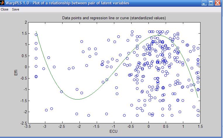
Nonlinear relationships provide a much more nuanced view of the data, but at the same time are much more difficult to interpret correctly. The graph below (click on it to enlarge) shows an S curve that is fitted to the data represented by the dots (or small circles) plotted in a scattered way on the graph. The latent variables are “ECU”, the extent to which electronic communication media are used by a team charged with developing a new product; and “Effi”, the efficiency of the team.

As you can see, the S curve is actually a combination of two U curves, one straight and the other inverted, connected at an inflection point. The inflection point is the point at the curve where the curvature, or second derivative of the S curve, changes direction. On the graph shown above, the inflection point is located at around minus 1 standard deviations from the "ECU" mean. That mean is at the zero mark on the horizontal axis.

Because an S curve is a combination of two U curves, we can interpret each U curve section separately. A straight U curve, like the one shown on the left side of the graph, before the inflection point, can be interpreted as follows.

The first half of the U curve goes from approximately minus 3.4 to minus 1.9 standard deviations from the mean, at which point the lowest team efficiency value is reached for the U curve. In that first half of the U curve, an increase in electronic communication media use leads to a decrease in team efficiency. After that first half, an increase in electronic communication media use leads to an increase in team efficiency.

One interpretation is that the first half of the U curve refers to novice users of electronic communication media. That is, novice users struggling to use more and more intensely communication media that they are not familiar with end up leading to efficiency losses for the team. At a certain point, around minus 1.9 standard deviations, that situation changes, and the teams start to really benefit from the use of electronic communication media, possibly because the second half of the U curve refers to users with more experience in using the media.

The interpretation of the second, inverted U curve, should be done in a similar fashion. As you can see, it is not easy to interpret nonlinear relationships. But the apparent simplicity of linear estimations of nonlinear relationships, which is usually what is done by other structural equation modeling software, is nothing but a mirage.

Field studies, small samples, and WarpPLS

Let us assume that a researcher wants to evaluate the effectiveness of new management method by conducting an intervention study in one single organization.

In this example, the researcher facilitates the use of a new management method by 20 managers in the organization, and then measures their degree of adoption of the method and their effectiveness.

The above is an example of a field study. Often field studies will yield small datasets, which will not conform to parametric analysis (e.g., ANOVA and ordinary multiple regression) pre-conditions. For example, the data will not typically be normally distributed.

WarpPLS can be very useful in the analysis of this type of data.

One reason is that, with small sample sizes, it may be difficult to identify linear relationships that are strong enough to be statistically significant (at P lower than 0.05, or less). Since WarpPLS implements nonlinear analysis algorithms, it can be very useful in the analysis of small samples.

Another reason is that P values are calculated through resampling, a nonparametric approach to statistical significance estimation. For small samples (i.e., lower than 100), jackknifing is the recommended resampling approach. Bootstrapping is recommended only for sample sizes greater than 100.

Geographically distributed collaborative SEM analysis using WarpPLS

I am currently conducting a geographically distributed collaborative SEM analysis using WarpPLS. The analysis involves a few people in different states of the USA, and two people outside the country. The collaborators are not only separated by large distances, but also operate in different time zones.

Yet, we have no problems collaborating. The collaboration is asynchronous – one person does some work one day, and shares it with the others, who review the work in the next few days and respond.

Since we all have WarpPLS installed on our computers, we exchange different versions of a WarpPLS project file (extension “.prj”) with the same dataset. This way we can do analyses in turns, and discuss the results on emails.

Each slightly different project file is saved with a different name – e.g., W3J_InfoOvld_2010_03_02.prj, W3B_InfoOvld_2010_03_02.prj, W2J_InfoOvld_2010_03_02.prj etc.

In the examples above, the first three letters indicate the SEM algorithm used (W3 = Warp3 PLS Regression; W2 = Warp2 PLS Regression), and the resampling method used (J = jackknifing; B = bootstrapping). The second part of the name describes the dataset, and the final part the date.

This is just one way of naming files. It works for our particular project, but more elaborate file names can be used in more complex collaborative SEM analyses.

This geographically distributed collaborative SEM analysis highlights one of the advantages of WarpPLS over other SEM software: all that is needed for the analysis is contained in one single project file.

Moreover, the project file will typically be only a few hundred kilobytes in size. In spite of its small size, the file includes the original data, and all of the results of the analysis.

One member of our team asked me how the project file can be so small. The reason is that all of the SEM analysis results are stored in a format that allows for their rendering every time they are viewed.

Plots of nonlinear relationships, for example, are not stored as bitmaps, but as equations that allow WarpPLS  to re-create those plots at the time of viewing.

Nonlinearity and type I and II errors in SEM analysis

Many relationships between variables studied in the natural and behavioral sciences seem to be nonlinear, often following a J-curve pattern (a.k.a. U-curve pattern). Other common relationships include the logarithmic, hyperbolic decay, exponential decay, and exponential. These and other relationships are modeled by WarpPLS.

Yet, the vast majority of statistical analysis methods used in the natural and behavioral sciences, from simple correlation analysis to structural equation modeling, assume relationships to be linear in the estimation of coefficients of association (e.g., Pearson correlations, standardized partial regression coefficients).

This may significantly distort results, especially in multivariate analyses, increasing the likelihood that researchers will commit type I and II errors in the same study. A type I error occurs in SEM analysis when an insignificant (the technical term is "non-significant") association is estimated as being significant (i.e., a “false positive”); a type II error occurs when a significant association is estimated as being insignificant (i.e., an existing association is “missed”).

The figure below shows a distribution of points typical of a J-curve pattern involving two variables, disrupted by uncorrelated error. The pattern, however, is modeled as a linear relationship. The line passing through the points is the best linear approximation of the distribution of points. It yields a correlation coefficient of .582. In this situation, the variable on the horizontal axis explains 33.9 percent of the variance of the variable on the vertical axis.

The figure below shows the same J-curve scatter plot pattern, but this time modeled as a nonlinear relationship. The curve passing through the points is the best nonlinear approximation of the distribution of the underlying J-curve, and excludes the uncorrelated error. That is, the curve does not attempt to model the uncorrelated error, only the underlying nonlinear relationship. It yields a correlation coefficient of .983. Here the variable on the horizontal axis explains 96.7 percent of the variance of the variable on the vertical axis.

WarpPLS transforms (or “warps”) J-curve relationship patterns like the one above BEFORE the corresponding path coefficients between each pair of variables are calculated. It does the same for many other nonlinear relationship patterns. In multivariate analyses, this may significantly change the values of the path coefficients, reducing the risk that researchers will commit type I and II errors.

The risk of committing type I and II errors is particularly high when: (a) a block of latent variables includes multiple predictor variables pointing and the same criterion variable; (b) one or more relationships between latent variables are significantly nonlinear; and (c) the predictor latent variables are correlated, even if they clearly measure different constructs (suggested by low variance inflation factors).

How is the warping done in WarpPLS?

WarpPLS does linear and nonlinear analyses. That is, users can set WarpPLS to estimate parameters based on a standard linear algorithm, and without any warping. They can also choose one of two nonlinear algorithms, thus taking advantage of the warping capabilities of the software.

In nonlinear analyses, what WarpPLS does is relatively simple at a conceptual level. It identifies a set of functions F1(LVp1), F2(LVp2) … that relate blocks of latent variable predictors (LVp1, LVp2 ...) to a criterion latent variable (LVc) in this way:

LVc = p1*F1(LVp1) + p2*F2(LVp2) + … + E.

In the equation above, p1, p2 ... are path coefficients, and E is the error term of the equation. All variables are standardized. Any model can be decomposed into a set of blocks relating latent variable predictors and criteria in this way.

In the Warp2 mode, the functions F1(LVp1), F2(LVp2) ... take the form of U curves (also known as J curves); defaulting to lines, if the relationships are linear. The term "U curve" is used here for simplicity, as noncyclical nonlinear relationships (e.g., exponential growth) can be represented through sections of straight or rotated U curves; the term "S curve" is also used here for simplicity.

In the Warp3 mode, the functions F1(LVp1), F2(LVp2) ... take the form of S curves; defaulting to U curves or lines, if the relationships follow U-curve patterns or are linear, respectively.

S curves are curves whose first derivative is a U curve. Similarly, U curves are curves whose first derivative is a line. U curves seem to be the most commonly found in natural and behavioral phenomena. S curves are also found, but apparently not as frequently as U curves.

U curves can be used to model most of the commonly seen functions in natural and behavioral studies, such as logarithmic, exponential, and hyperbolic decay functions. For these common types of functions, S-curve approximations will usually default to U curves.

Other types of curves beyond S curves might be found in specific types of situations, and require specialized analysis methods that are typically outside the scope of structural equation modeling. Examples are time series and Fourier analyses. Therefore these are beyond the scope of application of WarpPLS.

Typically, the more the functions F1(LVp1), F2(LVp2) ... look like curves, and unlike lines, the greater is the difference between the path coefficients p1, p2 ... and those that would have been obtained through a strictly linear analysis.

So, what WarpPLS does is not unlike what a researcher would do if he or she modified predictor latent variables prior to the calculation of path coefficients using a function like the logarithmic function. For example, as in the equation below, where a log transformation is applied to LVp1.

LVc = p1*log(LVp1) + p2*LVp2 + … + E.

However, WarpPLS does that automatically, and for a much wider range of functions, since a fairly wide range of functions can be modeled as U or S curves. Exceptions are complex trigonometric functions, where the dataset comprises many cycles. These require different methods to be properly modeled, such as the Fourier analyses methods mentioned above, and are usually outside the scope of structural equation modeling (SEM; which is the analysis method that WarpPLS automates).

Often the path coefficients p1, p2 ... will go up in value due to warped analysis, but that may not always be the case. Given the nature of multivariate analysis, an increase in a path coefficient may lead to a decrease in a path coefficient for an arrow pointing at the same criterion latent variable, because each path coefficient in a block is calculated in a way that controls for the effects of the other predictor latent variables.

Warped paths become significant in WarpPLS: YouTube video

Yet another new YouTube video is available for WarpPLS:

http://www.youtube.com/watch?v=_NQnVckeBb8

This video shows how path coefficients sometimes go up, and P values become significant, when warping takes place in a structural equation modeling (SEM) analysis using the software WarpPLS.

Since path coefficients are typically associated with hypotheses, which are supported if the paths are found to be significant, this will likely be music to many researchers' ears.

However, it is important to make two important points regarding this effect:

1. Path coefficients are not artificially inflated. They increase simply because the software is taking the nonlinear associations between latent variables into account when estimating path coefficients. Much like a researcher would apply a log(X) transformation to a predictor, before an ordinary regression analysis, if he or she knew that the predictor's relationship with a criterion variable Y was of the type Y=log(X).

2. Path coefficients do not always increase. Due to the nature of standardized partial regression coefficient calculation (the path coefficients, or betas, are standardized partial regression coefficients), when several predictor latent variables (LVs) point a one criterion LV, if one of the predictor LVs increases, some of the others predictor LVs may decrease as a result. In a sense, the predictor LVs "compete" for pieces of the space of variance explained for the criterion LV; if the predictor LVs are correlated, they tend "steal" variance space from each other (so to speak).

View nonlinear relationships in WarpPLS: YouTube video

A new Youtube video is available for WarpPLS:

http://www.youtube.com/watch?v=lHrTxWmM43A

This video shows how one can view nonlinear and linear relationships estimated through a structural equation modeling (SEM) analysis using the software WarpPLS.

The video also highlights one fact that makes software like WarpPLS particularly useful - most relationships in nature are nonlinear. This includes relationships in biology, business, sociology, physics etc.

As you will see in this video, the software shows a table with the types of relationships, warped or linear, between latent variables that are linked in the model. The term “warped” is used for relationships that are clearly nonlinear, and the term “linear” for linear or quasi-linear relationships. Quasi-linear relationships are slightly nonlinear relationships, which look linear upon visual inspection on plots of the regression curves that best approximate the relationships.

Plots with the points as well as the regression curves that best approximate the relationships can be viewed by clicking on a cell containing a relationship type description. These cells are the same as those that contain path coefficients, in the path coefficients table.

The plots of relationships between pairs of latent variables provide a much more nuanced view of how each pair of latent variables is related. However, caution must be taken in the interpretation of these plots, especially when the distribution of data points is very uneven.

An extreme example would be a warped plot in which all of the data points would be concentrated on the right part of the plot, with only one data point on the far left part of the plot. That single data point, called an outlier, would influence the shape of the nonlinear relationship. In these cases, the researcher must decide whether the outlier is “good” data that should be allowed to shape the relationship, or is simply “bad” data resulting from a data collection error.