Interpreting the U and S curves generated by WarpPLS

Linear relationships between pairs of latent variables, that is, those relationships best described by a line, are relatively easy to interpret. They suggest that an increase in one variable either leads to an increase (if the slope of the line is positive) or decrease (if the slope is negative) in the other variable.

Nonlinear relationships provide a much more nuanced view of the data, but at the same time are much more difficult to interpret correctly. The graph below (click on it to enlarge) shows an S curve that is fitted to the data represented by the dots (or small circles) plotted in a scattered way on the graph. The latent variables are “ECU”, the extent to which electronic communication media are used by a team charged with developing a new product; and “Effi”, the efficiency of the team.

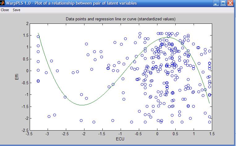
As you can see, the S curve is actually a combination of two U curves, one straight and the other inverted, connected at an inflection point. The inflection point is the point at the curve where the curvature, or second derivative of the S curve, changes direction. On the graph shown above, the inflection point is located at around minus 1 standard deviations from the "ECU" mean. That mean is at the zero mark on the horizontal axis.

Because an S curve is a combination of two U curves, we can interpret each U curve section separately. A straight U curve, like the one shown on the left side of the graph, before the inflection point, can be interpreted as follows.

The first half of the U curve goes from approximately minus 3.4 to minus 1.9 standard deviations from the mean, at which point the lowest team efficiency value is reached for the U curve. In that first half of the U curve, an increase in electronic communication media use leads to a decrease in team efficiency. After that first half, an increase in electronic communication media use leads to an increase in team efficiency.

One interpretation is that the first half of the U curve refers to novice users of electronic communication media. That is, novice users struggling to use more and more intensely communication media that they are not familiar with end up leading to efficiency losses for the team. At a certain point, around minus 1.9 standard deviations, that situation changes, and the teams start to really benefit from the use of electronic communication media, possibly because the second half of the U curve refers to users with more experience in using the media.

The interpretation of the second, inverted U curve, should be done in a similar fashion. As you can see, it is not easy to interpret nonlinear relationships. But the apparent simplicity of linear estimations of nonlinear relationships, which is usually what is done by other structural equation modeling software, is nothing but a mirage.

Viewing and changing settings in WarpPLS 1.0 and 2.0

The blog post below refers to version 1.0 - 2.0 of WarpPLS. See this YouTube video on how to view and change settings for version 3.0. For more recent versions, see the WarpPLS User Manual and YouTube videos available from warppls.com.

***

The view or change settings window (see figure below, click on it to enlarge) allows you to select an algorithm for the SEM analysis, select a resampling method, and select the number of resamples used, if the resampling method selected was bootstrapping. The analysis algorithms available are Warp3 PLS Regression, Warp2 PLS Regression, PLS Regression, and Robust Path Analysis.

Many relationships in nature, including relationships involving behavioral variables, are nonlinear and follow a pattern known as U-curve (or inverted U-curve). In this pattern a variable affects another in a way that leads to a maximum or minimum value, where the effect is either maximized or minimized, respectively. This type of relationship is also referred to as a J-curve pattern; a term that is more commonly used in economics and the health sciences.

The Warp2 PLS Regression algorithm tries to identify a U-curve relationship between latent variables, and, if that relationship exists, the algorithm transforms (or “warps”) the scores of the predictor latent variables so as to better reflect the U-curve relationship in the estimated path coefficients in the model. The Warp3 PLS Regression algorithm, the default algorithm used by the software, tries to identify a relationship defined by a function whose first derivative is a U-curve. This type of relationship follows a pattern that is more similar to an S-curve (or a somewhat distorted S-curve), and can be seen as a combination of two connected U-curves, one of which is inverted.

The PLS Regression algorithm does not perform any warping of relationships. It is essentially a standard PLS regression algorithm, whereby indicators’ weights, loadings and factor scores (a.k.a. latent variable scores) are calculated based on a least squares minimization sub-algorithm, after which path coefficients are estimated using a robust path analysis algorithm. A key criterion for the calculation of the weights, observed in virtually all PLS-based algorithms, is that the regression equation expressing the relationship between the indicators and the factor scores has an error term that equals zero. In other words, the factor scores are calculated as exact linear combinations of their indicators. PLS regression is the underlying weight calculation algorithm used in both Warp3 and Warp2 PLS Regression. The warping takes place during the estimation of path coefficients, and after the estimation of all weights and loadings in the model. The weights and loadings of a model with latent variables make up what is often referred to as outer model, whereas the path coefficients among latent variables make up what is often called the inner model.

Finally, the Robust Path Analysis algorithm is a simplified algorithm in which factor scores are calculated by averaging all of the indicators associated with a latent variable; that is, in this algorithm weights are not estimated through PLS regression. This algorithm is called “Robust” Path Analysis, because, as with most robust statistics methods, the P values are calculated through resampling. If all latent variables are measured with single indicators, the Robust Path Analysis and the PLS Regression algorithms will yield identical results.

One of two resampling methods may be selected: bootstrapping or jackknifing. Bootstrapping, the software’s default, is a resampling algorithm that creates a number of resamples (a number that can be selected by the user), by a method known as “resampling with replacement”. This means that each resample contains a random arrangement of the rows of the original dataset, where some rows may be repeated. (The commonly used analogy of a deck of cards being reshuffled, leading to many resample decks, is a good one, but not entirely correct because in bootstrapping the same card may appear more than once in each of the resample decks.) Jacknifing, on the other hand, creates a number of resamples that equals the original sample size, and each resample has one row removed. That is, the sample size of each resample is the original sample size minus 1. Thus, the choice of number of resamples has no effect on jackknifing, and is only relevant in the context of bootstrapping.

How is the warping done in WarpPLS?

WarpPLS does linear and nonlinear analyses. That is, users can set WarpPLS to estimate parameters based on a standard linear algorithm, and without any warping. They can also choose one of two nonlinear algorithms, thus taking advantage of the warping capabilities of the software.

In nonlinear analyses, what WarpPLS does is relatively simple at a conceptual level. It identifies a set of functions F1(LVp1), F2(LVp2) … that relate blocks of latent variable predictors (LVp1, LVp2 ...) to a criterion latent variable (LVc) in this way:

LVc = p1*F1(LVp1) + p2*F2(LVp2) + … + E.

In the equation above, p1, p2 ... are path coefficients, and E is the error term of the equation. All variables are standardized. Any model can be decomposed into a set of blocks relating latent variable predictors and criteria in this way.

In the Warp2 mode, the functions F1(LVp1), F2(LVp2) ... take the form of U curves (also known as J curves); defaulting to lines, if the relationships are linear. The term "U curve" is used here for simplicity, as noncyclical nonlinear relationships (e.g., exponential growth) can be represented through sections of straight or rotated U curves; the term "S curve" is also used here for simplicity.

In the Warp3 mode, the functions F1(LVp1), F2(LVp2) ... take the form of S curves; defaulting to U curves or lines, if the relationships follow U-curve patterns or are linear, respectively.

S curves are curves whose first derivative is a U curve. Similarly, U curves are curves whose first derivative is a line. U curves seem to be the most commonly found in natural and behavioral phenomena. S curves are also found, but apparently not as frequently as U curves.

U curves can be used to model most of the commonly seen functions in natural and behavioral studies, such as logarithmic, exponential, and hyperbolic decay functions. For these common types of functions, S-curve approximations will usually default to U curves.

Other types of curves beyond S curves might be found in specific types of situations, and require specialized analysis methods that are typically outside the scope of structural equation modeling. Examples are time series and Fourier analyses. Therefore these are beyond the scope of application of WarpPLS.

Typically, the more the functions F1(LVp1), F2(LVp2) ... look like curves, and unlike lines, the greater is the difference between the path coefficients p1, p2 ... and those that would have been obtained through a strictly linear analysis.

So, what WarpPLS does is not unlike what a researcher would do if he or she modified predictor latent variables prior to the calculation of path coefficients using a function like the logarithmic function. For example, as in the equation below, where a log transformation is applied to LVp1.

LVc = p1*log(LVp1) + p2*LVp2 + … + E.

However, WarpPLS does that automatically, and for a much wider range of functions, since a fairly wide range of functions can be modeled as U or S curves. Exceptions are complex trigonometric functions, where the dataset comprises many cycles. These require different methods to be properly modeled, such as the Fourier analyses methods mentioned above, and are usually outside the scope of structural equation modeling (SEM; which is the analysis method that WarpPLS automates).

Often the path coefficients p1, p2 ... will go up in value due to warped analysis, but that may not always be the case. Given the nature of multivariate analysis, an increase in a path coefficient may lead to a decrease in a path coefficient for an arrow pointing at the same criterion latent variable, because each path coefficient in a block is calculated in a way that controls for the effects of the other predictor latent variables.