PLS Applications Symposium; 12-14 April 2023; Laredo, Texas

PLS Applications Symposium; 12-14 April 2023; Laredo, Texas
(Abstract submissions accepted until 17 February 2023)

*** Attendance (face-to-face or online) ***

The Symposium will be conducted as part of the multidisciplinary Annual Western Hemispheric Trade Conference, organized by the Center for the Study of Western Hemispheric Trade. Our workshop in PLS-SEM will be conducted entirely online. Our expectation is that participants will be allowed to attend Conference sessions either face-to-face or online.

When indicating the type of their submission, participants should indicate whether they intend to attend face-to-face or online. This should be done within parentheses after indicating the submission type. For example - "Type of submission: Presentation (online)".

*** Only abstracts are needed for the submissions ***

The partial least squares (PLS) method has increasingly been used in a variety of fields of research and practice, particularly in the context of PLS-based structural equation modeling (SEM). The focus of this Symposium is on the application of PLS-based methods, from a multidisciplinary perspective. For types of submissions, deadlines, and other details, please visit the Symposium’s web site:

https://plsas.net

*** Workshop on PLS-SEM ***

On 12 April 2023 a full-day workshop on PLS-SEM will be conducted by Dr. Ned Kock and Dr. Geoffrey Hubona, using the software WarpPLS. Dr. Kock is the original developer of this software, which is one of the leading PLS-SEM tools today; used by thousands of researchers from a wide variety of disciplines, and from many different countries. Dr. Hubona has extensive experience conducting research and teaching topics related to PLS-SEM, using WarpPLS and a variety of other tools. This workshop will be hands-on and interactive, and will have two parts: (a) basic PLS-SEM issues, conducted in the morning (9 am - 12 noon) by Dr. Hubona; and (b) intermediate and advanced PLS-SEM issues, conducted in the afternoon (2 pm - 5 pm) by Dr. Kock. Participants may attend either one, or both of the two parts.

The following topics, among others, will be covered - Running a Full PLS-SEM Analysis - Conducting a Moderating Effects Analysis - Viewing Moderating Effects via 3D and 2D Graphs - Creating and Using Second Order Latent Variables - Viewing Indirect and Total Effects - Viewing Skewness and Kurtosis of Manifest and Latent Variables - Viewing Nonlinear Relationships - Solving Collinearity Problems - Conducting a Factor-Based PLS-SEM Analysis - Using Consistent PLS Factor-Based Algorithms - Exploring Statistical Power and Minimum Sample Sizes - Exploring Conditional Probabilistic Queries - Exploring Full Latent Growth - Conducting Multi-Group Analyses - Assessing Measurement Invariance - Creating Analytic Composites.

-----------------------------------------------------------
Ned Kock
Symposium Chair
https://plsas.net

Model-driven data analytics (MDDA): Resources for teachers and students

The technique of model-driven data analytics (MDDA) involves the creation of a path model expressing an applied theory, and testing the model using path analysis with latent variables. The latter, path analysis with latent variables, is generally known as structural equation modeling (SEM).

MDDA emerged from the work of a special category of users of the software WarpPLS – data analysis consultants, who regularly work with organizations to provide data-driven recommendations.

While MDDA can be implemented through a variety of software tools, it has found wide adoption among WarpPLS users, because of the many powerful features of this software that can be used in this context. Moreover, in WarpPLS all analyses are model-driven, which makes this software much more user-friendly than other software tools that rely on extensive scripting to conduct analyses.

The website linked below provides several resources for teachers and students, including: a textbook, which may be used by teachers of university courses on MDDA, as a free online document; datasets, which include not only data, but also scenarios, questions, and variables (these are used to illustrate how MDDA can be used to address the needs of various organizations); and YouTube videos, which provide step-by-step illustrations of how to analyze data in the context of scenarios, questions, and variables.

https://scriptwarp.com/mdda

Best regards to all!

A thank you note to the workshop participants at The University of Texas at El Paso

This is just at thank you note to the College of Business Administration at The University of Texas at El Paso for hosting me on 10-11 November 2022 for a workshop on SEM using the software WarpPLS.

Special thanks go to Dr. Kevin Dow, his wonderful team at the Accounting and Information Systems Department, and those who participated in the workshop.

Several of the participants had quite a great deal of expertise in SEM and WarpPLS. It was a joy to conduct the workshop, and answer some very insightful questions!

Thank you and best regards to all!

Ned Kock
https://nedkock.com

Dichotomous variables

There are several ways in which a model with an endogenous dichotomous variable can be analyzed in PLS-SEM - via the logistic regression variables technique, without any additional treatment, and via the conditional probabilistic queries technique. Below we discuss the first two options.

Logistic regression variables technique

Starting in version 8.0 of WarpPLS, the menu option “Explore logistic regression” allows you to create a logistic regression variable as a new indicator that has both unstandardized and standardized values. Logistic regression is normally used to convert an endogenous variable on a non-ratio scale (e.g., dichotomous) into a variable reflecting probabilities. You need to choose the variable to be converted, which should be an endogenous variable, and its predictors. 

The new logistic regression variable is meant to be used as a replacement for the endogenous variable on which it is based. Two algorithms are available: probit and logit. The former is recommended for dichotomous variables; the latter for non-ratio variables where the number of different values (a.k.a. “distinct observations”) is greater than 2 but still significantly smaller than the sample size; e.g., 10 different values over a sample size of 100. The unstandardized values of a logistic regression variable are probabilities; going from 0 to 1. 

Since a logistic regression variable can be severely collinear with its predictors, you can set a local full collinearity VIF cap for the logistic regression variable. Predictor-criterion collinearity, or lateral collinearity, is rarely assessed or controlled in classic logistic regression algorithms. 

For more on this topic, see the links below.

Explore Logistic Regression in WarpPLS

https://youtu.be/PO65ySuhPW0

Using Logistic Regression in PLS-SEM with Composites and Factors

https://youtu.be/c9ySXN4NVus

Without any additional treatment

Models with dichotomous endogenous variables can also be tested with WarpPLS without any additional treatment, although this may lead to path coefficient suppression as well as other problems. Based on preliminary Monte Carlo simulations, the following combination of algorithm and P value calculation method seems to be the most advisable, if users want to analyze models with composite-based algorithms: PLS regression and stable.

Below is a model with a dichotomous dependent variable - Effe. The variable assumes two values, 0 or 1, to reflect low or high levels of "effectiveness".

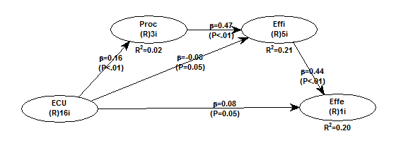
The graph below shows the expected values of Effe given Effi. The latter is one of the LVs that point at Effe in the model. The values of Effe and Effi are unstandardized.

Arguably a model with a dichotomous dependent variable cannot be viably tested with ordinary multiple regression because the dependent variable is not normally distributed (as it assumes only two values).

The graph below shows a histogram with the distribution of values of Effe. This variable's skewness is -0.423 and excess kurtosis is -1.821.

This is not a problem for WarpPLS because P values are calculated via nonparametric techniques that do not assume in their underlying design that any variables in the model meet parametric expectations; such as the expectations of univariate and multivariate unimodality and normality.

If a dependent variable refers to a probability (as in logistic regression), and is expected to be associated with a predictor according to a logistic function, you should use the Warp3 or Warp3 basic inner model algorithms to relate the two variables.

Model with endogenous dichotomous variable

There are two main ways in which a model with an endogenous dichotomous variable can be analyzed in PLS-SEM - via the logistic regression variables technique, and via the conditional probabilistic queries technique.

Logistic regression variables technique

Starting in version 8.0 of WarpPLS, the menu option “Explore logistic regression” allows you to create a logistic regression variable as a new indicator that has both unstandardized and standardized values. Logistic regression is normally used to convert an endogenous variable on a non-ratio scale (e.g., dichotomous) into a variable reflecting probabilities. You need to choose the variable to be converted, which should be an endogenous variable, and its predictors. 

The new logistic regression variable is meant to be used as a replacement for the endogenous variable on which it is based. Two algorithms are available: probit and logit. The former is recommended for dichotomous variables; the latter for non-ratio variables where the number of different values (a.k.a. “distinct observations”) is greater than 2 but still significantly smaller than the sample size; e.g., 10 different values over a sample size of 100. The unstandardized values of a logistic regression variable are probabilities; going from 0 to 1. 

Since a logistic regression variable can be severely collinear with its predictors, you can set a local full collinearity VIF cap for the logistic regression variable. Predictor-criterion collinearity, or lateral collinearity, is rarely assessed or controlled in classic logistic regression algorithms. 

For more on this topic, see the links below.

Explore Logistic Regression in WarpPLS

https://youtu.be/PO65ySuhPW0

Using Logistic Regression in PLS-SEM with Composites and Factors

https://youtu.be/c9ySXN4NVus

Conditional probabilistic queries technique

How do we interpret the results of a model with an endogenous dichotomous variable, using the conditional probabilistic queries technique? Let us use the model below to illustrate the answer to this question. In this model we have one endogenous dichotomous variable “Success” that is significantly caused in a direct way by two predictors: “Projmgt” and “JSat”. The direct effect of a third predictor, namely "ECollab", is relatively small and borderline significant.

Let us assume that the unit of analysis is a team of people. The variable “Success” is coded as 0 or 1, meaning that a team is either successful or not. After standardization, the 0 and 1 will be converted into a negative and a positive number. The standardized version of the variable “Success” will have a mean of zero and a standard deviation of 1.

One way to interpret the results is the following. The probability that a team will be successful (i.e., that “Success” > 0) is significantly affected by increases in the variables “Projmgt” and “JSat”.

WarpPLS users are able, starting in version 6.0, to calculate conditional probabilities as shown below, without having to resort to transformations based on assumed underlying functions, such as those performed by logistic regression. In this screen shot, only latent variables are used, and they are all assumed to be standardized.

In the screen shot above, we can see that the probability that a team will be successful (i.e., that “Success” > 0), if “Projmgt” > 1 and “JSat” > 1, is 52.2 percent. Stated differently, if “Projmgt” and “JSat” are high (greater than 1 standard deviation above the mean), then the probability of success is slightly greater than chance.

A probability of 52.2 percent is not that high. The reason why it is not higher, in the context of the conditional probabilistic query above, is that we are not including the variable "ECollab" in the mix. Still, it does not seem like “Projmgt” and “JSat” being high are sufficient conditions for success, although they may be necessary conditions.

Consider a different set of conditional probabilities. If a team is successful (i.e., if “Success” > 0), what is the probability that “Projmgt” and “JSat” are low for that team. The answer, shown in the screen below, is 1.3 percent. That is a very low probability, suggesting that “Projmgt” and “JSat” matter as necessary but not sufficient elements for success.

These are among the conditional probabilistic queries that users are able to make starting in version 6.0 of WarpPLS. Bayes’ theorem is used to produce the answers to the queries.

Using causality assessment indices in PLS-SEM

The article below discusses how one can use causality assessment indices, to assess the network of causal links in a model, in the context of structural equation modeling via partial least squares (PLS-SEM).

Kock, N. (2022). Using causality assessment indices in PLS-SEM. Data Analysis Perspectives Journal, 3(5), 1-6.

Link to full-text file for this and other DAPJ articles:

https://scriptwarp.com/dapj/#Published_Articles

Abstract:

We discuss the use of four causality assessment indices, through an illustrative model analyzed with WarpPLS, a leading software tool for structural equation modeling via partial least squares (PLS-SEM). The indices are the: Simpson's paradox ratio (SPR), R-squared contribution ratio (RSCR), statistical suppression ratio (SSR), and nonlinear bivariate causality direction ratio (NLBCDR). We provide an example of how the causality assessment indices can be presented in a journal article, conference paper, or other research report document.

Best regards to all!

Possible installation problems and the MATLAB Compiler Runtime

The vast majority of WarpPLS users do not have any installation problems, but some users do. One possible cause is an incompatibility between the MATLAB Compiler Runtime and their computer's operating system setup. This is explored in more detail below.

Another possible cause of installation problems is one or more software applications that interfere with the proper running of WarpPLS. There have been reports from users suggesting that the following software applications may do that: Panda Antivirus, Norton Antivirus, and XLSTAT.

Yet another possible cause of installation problems are security software tools (to stop malware) that prevent users from making modifications in the folders in their computers that store data about programs. Closely aligned with this cause are security restrictions placed on computers by their organizations' IT offices.

The MATLAB Compiler Runtime

The MATLAB Compiler Runtime is for MATLAB programs what the Java Runtime is for Java programs, and what the Microsoft .NET Framework is for .NET-based programs. That is, it is a set of executable modules that are called by executable files compiled using MATLAB.

WarpPLS is an executable file compiled using MATLAB, and thus requires the MATLAB Compiler Runtime (version 7.14) to run properly. Like many other runtime libraries, the MATLAB Compiler Runtime has originally been developed in C and C++.

MATLAB does not have to be installed for WarpPLS to run

The MATLAB Compiler Runtime is provided in the self-extracting executable file used for the installation of WarpPLS. It is free of charge. MATLAB does not have to be installed for WarpPLS to run, only the specific MATLAB Compiler Runtime that accompanies WarpPLS.

In theory, the MATLAB Compiler Runtime should allow for a “compile once, run everywhere” approach to programming. That is, code that uses the MATLAB Compiler Runtime would be developed on one operating system, compiled, and then deployed, together with the MATLAB Compiler Runtime, to computers running any operating system.

This approach works well in theory, but not always in practice. This comment applies not only to MATLAB but also to Java and .NET applications – you are probably well aware of this if you are a Java or .NET programmer.

Seek professional IT support if you are using an organizational computer

It is possible that a specific user’s computer configuration will prevent the proper installation of the MATLAB Compiler Runtime, by blocking certain operating system configuration changes (e.g., Windows registry changes), as a security measure. This is often the case when organizational computers are used.

Also, a user may not have administrator rights on a computer, or have limited administrator/power user rights, which may prevent certain operating system configuration changes necessary for the proper installation of the MATLAB Compiler Runtime. Having professional IT support in this type of scenario is a must.

Here are a few steps to take if you are having problems installing and running WarpPLS on a Windows computer:

1) Run WarpPLS as administrator.

Some users solved their installation problems by simply doing this: Right-clicking on the WarpPLS icon and choosing the option to run it as administrator.

2) Reinstall WarpPLS using the larger file containing the MATLAB Compiler Runtime (approximately 170 MB), choosing the option “Repair”.

There have been reported cases in which users cannot start WarpPLS or move beyond WarpPLS’s first screen. This may happen even if the user has a valid license, with the software behaving as though it is not licensed at all. This may also happen before the user acquires a valid license, while trying to use WarpPLS within the trial license period.

A possible solution here that has worked well in the past is to reinstall WarpPLS using the larger file containing the MATLAB Compiler Runtime. When the MATLAB Compiler Runtime installation software pops up, choose the option “Repair”, and proceed with the full reinstallation.

3) Do the above, but change the folder where the WarpPLS program is installed, choosing a folder that is not in a protected area.

As a possible variation to the above, you may change the folder where the WarpPLS program is installed, choosing a folder that is not in a protected area. For example, you may choose the folder “C:\WarpPLS” or the folder “C:\WarpPLS [version]”. Being outside a protected area prevents certain software, such as antivirus software and malware, from interfering with WarpPLS’s execution.

4) Completely uninstall the MATLAB Compiler Runtime and WarpPLS, disable any antivirus software currently running, reinstall the MATLAB Compiler Runtime and WarpPLS, and then re-enable the antivirus software.

To uninstall the MATLAB Compiler Runtime, follow the following procedure (or a similar procedure, depending on the version of Windows you are using): go the “Control Panel”, click on “Add or Remove Programs” or “Programs and Features”, and uninstall the MATLAB Compiler Runtime.

To uninstall the main software program (i.e., WarpPLS), simply delete the main software installation folder. This folder is usually “C:\Program Files\WarpPLS [version]” or “C:\Program Files (x86)\WarpPLS [version]”, unless you chose a different folder for the main software program during the installation process. Then delete the shortcut created by the software from the desktop.

5) Check the "Program Files" and the "Program Files (x86)" directories (assuming that the MATLAB Compiler Runtime is installed on the C drive), to see if one of the following folders is there.

C:\Program Files\MATLAB\MATLAB Compiler Runtime\v714\runtime\win32

C:\Program Files (x86)\MATLAB\MATLAB Compiler Runtime\v714\runtime\win32

If not, make sure that you are logged into your computer with full administrator rights, and reinstall the MATLAB Compiler Runtime. You can do that running the self-installing .exe file (approximately 170 MB) for WarpPLS, which includes the MATLAB Compiler Runtime. Or, contact your local IT support, and ask them to help you do so.

6) Go to the Command Prompt and type “PATH”, to see if one of the following paths shows on the list provided.

C:\Program Files\MATLAB\MATLAB Compiler Runtime\v714\runtime\win32

C:\Program Files (x86)\MATLAB\MATLAB Compiler Runtime\v714\runtime\win32

If not, on the Command Prompt, type one of the following commands, depending on the folder in which the MATLAB Compiler Runtime is installed:

set PATH=C:\Program Files\MATLAB\MATLAB Compiler Runtime\v714\runtime\win32;%PATH%

set PATH=C:\Program Files (x86)\MATLAB\MATLAB Compiler Runtime\v714\runtime\win32;%PATH%

Then type “PATH” again, and make sure that the new path has been added. This will change the Windows registry; a minor and pretty harmless change. If you are concerned about making registry changes yourself, or cannot do that due to limited rights or any other reason, please contact your local IT support, and ask them to help you do so.

7) Try to install WarpPLS on a different computer, and see if it runs well there.

This last step is annoying but important because there are certain computer-specific configuration setups, or even malware allowed in by those setups, that may prevent the MATLAB Compiler Runtime from properly installing or executing. This is rare, but does happen sometimes. Comparing computers can help solve problems like these.

If you can install and run WarpPLS on one computer, but not on another, there may be a computer configuration or malware problem that is preventing you from doing so. If you have access to good-quality local IT support, you should contact it, and ask them to help you identify and solve the problem.

A thank you note to the participants in the 2022 PLS Applications Symposium

This is just a thank you note to those who participated, either as presenters or members of the audience, in the 2022 PLS Applications Symposium:

https://plsas.net/

As in previous years, it seems that it was a good idea to run the Symposium as part of the Western Hemispheric Trade Conference. This allowed attendees to take advantage of a subsidized registration fee, and also participate in other Conference sessions and the Conference's social event.

I have been told that the proceedings will be available soon, if they are not available yet, from the Western Hemispheric Trade Conference web site, which can be reached through the Symposium web site (link above).

Also, we had a nice full-day workshop on PLS-SEM using the software WarpPLS. This workshop, conducted by Dr. Jeff Hubona and myself, was fairly hands-on and interactive. Some participants had quite a great deal of expertise in PLS-SEM and WarpPLS. It was a joy to conduct the workshop!

As soon as we define the dates, we will be announcing next year’s PLS Applications Symposium. Like this years’ Symposium, it will take place in Laredo, Texas, probably in the first half of April as well.

Thank you and best regards to all!

-----------------------------------------------------------
Ned Kock
Symposium Chair
https://plsas.net/

WarpPLS 8.0 upgraded to stable: Logistic regression, full latent growth graphs, HTMT2 ratios, and more!

Dear colleagues:

Version 8.0 of WarpPLS is now available as a stable version. You can download and install it for a free trial from:

https://warppls.com

Each new version of the software incorporates features that aim at achieving an important end goal: to allow users to employ SEM to conduct any of the major statistical tests; from relatively simple tests such as comparisons of means, to more sophisticated ones such as nonlinear SEM tests employing logistic regression. Among the community of users of this software, there are very sophisticated SEM experts that constantly challenge us to implement new data analysis features, as well as to make the existing features as easy to use as possible. Because of the constant input from our users, including those who are very knowledgeable about SEM, the software now arguably provides the most extensive set of features of any SEM software. We hope to continue in this path as the SEM field evolves. Below we outline new features added to the current version of the software.

Logistic regression variables. The menu option “Explore logistic regression” now allows you to create a logistic regression variable as a new indicator that has both unstandardized and standardized values. Logistic regression is normally used to convert an endogenous variable on a non-ratio scale (e.g., dichotomous) into a variable reflecting probabilities. You need to choose the variable to be converted, which should be an endogenous variable, and its predictors. The new logistic regression variable is meant to be used as a replacement for the endogenous variable on which it is based. Two algorithms are available: probit and logit. The former is recommended for dichotomous variables; the latter for non-ratio variables where the number of different values (a.k.a. “distinct observations”) is greater than 2 but still significantly smaller than the sample size; e.g., 10 different values over a sample size of 100. The unstandardized values of a logistic regression variable are probabilities; going from 0 to 1. Since a logistic regression variable can be severely collinear with its predictors, you can set a local full collinearity VIF cap for the logistic regression variable. Predictor-criterion collinearity, or lateral collinearity (Kock & Lynn, 2012), is rarely assessed or controlled in classic logistic regression algorithms.

Absolute and relative variation measures. You can now view the number of different values (a.k.a. “distinct observations”) for all indicators and latent variables, as well as the ratio between the number of different values and sample size. The first is an absolute and the second a relative variation measure. These are available under the menu options “View or save correlations and descriptive statistics for indicators” and “View latent variable coefficients”, respectively. These measures can help inform decisions about whether to use logistic regression, particularly in connection with endogenous latent variables. If the number of different values is significantly smaller than the sample size (e.g., 10 different values over a sample size of 100) for an endogenous latent variable, that means that a new logistic regression variable could be created and used as a replacement for the endogenous variable. If several predictors are available, the new logistic regression variable will incorporate more variation than the endogenous variable on which it is based, which will typically be reflected in larger coefficients of association (e.g., path coefficients) when the logistic regression variable is used in the model.

Graphs for full latent growth coefficients. You can now view several graphs for each of the full latent growth coefficients provided under the menu option “Explore full latent growth”. Full latent growth coefficients have a number of applications, such as: moderating effects analyses, nonlinearity tests, multi-group and measurement invariance tests, and the assessment of moderated mediation effects. Each of the graphs is made up of several plots, which refer to changes in the coefficients selected (e.g., path coefficients) for the relationship between the variables shown in the X and Y axes, as the latent growth variable goes from low to high. The following graph menu options are available: “Full sample splits (megaphones)”, “Partial sub-samples splits (megaphones)”, “Full sample splits (bars)”, “Partial sub-samples splits (bars)”, “Full sample splits (lines)”, and “Partial sub-samples splits (lines)”.

HTMT2 ratios. The sub-option “'Discriminant validity coefficients (extended set)”, under the menu option “Explore additional coefficients and indices”, now allows you to inspect the newest version of the set of heterotrait-monotrait (HTMT) ratios calculated by the software. These have been dubbed HTMT2 ratios. The HTMT and HTMT2 ratios have been proposed for discriminant validity assessment, particularly in the context of composite-based SEM via classic PLS algorithms; as opposed to factor-based SEM via modern algorithms that estimate factors (which have been available from this software for quite some time now). Discriminant validity is a measure of the quality of a measurement instrument; the instrument itself is typically a set of question-statements. A measurement instrument has good discriminant validity if the question-statements (or other measures) associated with each latent variable are not confused by the respondents, in terms of their meaning, with the question-statements associated with other latent variables.

Incremental interface improvement. This is conducted in each new version of the software. At several points the code has been modified so that the user interface experiences are improved. This has led in several cases to what appears to be a smoother flow through the several steps and procedures guided by the user interface. Several elements of the graphical user interface, such as screens and warning messages, have been optimized so that users can perform SEM analysis tasks with only a few clicks – and in a straightforward fashion. Nevertheless, care is always taken to ensure that the user interfaces do not change too much, otherwise users would have to re-learn how to use the interface whenever a new version is released.

Incremental code optimization. This is also conducted in each new version of the software. At several points the code has been optimized for speed, stability, and coefficient estimation precision. In some cases, the optimization has led to lesser propagation of sampling error, making the software reach accurate results at lower sample sizes – that is, increasing the statistical efficiency of the software. These incremental code optimization changes have led to incremental gains in speed even as new features have been added. More often than not, new features require additional computational steps and often complex calculations, mostly to generate internal checks and coefficients that were not available before.

Take a look at the following videos, which have been created using this new version. They illustrate the new features outlined above.

Explore Logistic Regression in WarpPLS

View the Number of Different Values for Variables in WarpPLS

View Full Latent Growth Graphs in WarpPLS

Holistic Measurement Model Assessment in SEM with WarpPLS

Reduce Common Structural Variation with WarpPLS

Assessing Multiple Reciprocal Relationships in SEM with WarpPLS

Choose the Correlation Signs for Anchor Variables in a Multilevel Analysis with WarpPLS

Using Logistic Regression in PLS-SEM with Composites and Factors

Conducting a What-if Analysis in PLS-SEM with Analytic Composites

Reference:

Kock, N., & Lynn, G. (2012). Lateral collinearity and misleading results in variance-based SEM: An illustration and recommendations. Journal of the Association for Information Systems, 13(7), 546-580.

Best regards to all!

Minimum sample size estimation in SEM: Contrasting results for models using composites and factors

The article below discusses how one can conduct a minimum sample size estimation, contrasting results for models using composites and factors, in the context of structural equation modeling via partial least squares (PLS-SEM).

Ezeugwa, B., Talukder, M. F., Amin, M. R., Hossain, S. I., & Arslan, F. (2022). Minimum sample size estimation in SEM: Contrasting results for models using composites and factors. Data Analysis Perspectives Journal, 3(4), 1-7.

Link to full-text file for this and other DAPJ articles:

https://scriptwarp.com/dapj/#Published_Articles

Abstract:

Estimating the minimum required sample size is an essential issue for studies that use structural equation modeling employing partial least squares (PLS-SEM). Several PLS-SEM-based studies ignore this critical step or use simple techniques, which lead to inaccurate sample size estimations. This paper illustrates two effective heuristic methods to estimate the minimum required sample size using WarpPLS, a leading PLS-SEM software tool.

Best regards to all!

Testing and controlling for endogeneity in PLS-SEM with stochastic instrumental variables

The article below discusses a procedure that can be used to simultaneously test and control for endogeneity, in the context of structural equation modeling via partial least squares (PLS-SEM).

Kock, N. (2022). Testing and controlling for endogeneity in PLS-SEM with stochastic instrumental variables. Data Analysis Perspectives Journal, 3(3), 1-6.

Link to full-text file for this and other DAPJ articles:

https://scriptwarp.com/dapj/#Published_Articles

Abstract:

We discuss a procedure that can be used to simultaneously test and control for endogeneity in models analyzed with structural equation modeling via partial least squares (PLS-SEM). It relies on the creation of stochastic instrumental variables for endogenous latent variables, and their use as control variables. The procedure can be seen as an implementation of the Durbin–Wu–Hausman test, often referred to as the Hausman test, with stochastic instrumental variables. It can also be seen as a generalization of the two-stage least squares procedure. We illustrate the procedure with WarpPLS, a leading PLS-SEM tool.

Best regards to all!

WarpPLS 8.0 beta now available: Logistic regression, full latent growth graphs, HTMT2 ratios, and more!

Dear colleagues:

Version 8.0 of WarpPLS is now available, as a beta version. You can download and install it for a free trial from:

https://warppls.com

Each new version of the software incorporates features that aim at achieving an important end goal: to allow users to employ SEM to conduct any of the major statistical tests; from relatively simple tests such as comparisons of means, to more sophisticated ones such as nonlinear SEM tests employing logistic regression. Among the community of users of this software, there are very sophisticated SEM experts that constantly challenge us to implement new data analysis features, as well as to make the existing features as easy to use as possible. Because of the constant input from our users, including those who are very knowledgeable about SEM, the software now arguably provides the most extensive set of features of any SEM software. We hope to continue in this path as the SEM field evolves. Below we outline new features added to the current version of the software.

Logistic regression variables. The menu option “Explore logistic regression” now allows you to create a logistic regression variable as a new indicator that has both unstandardized and standardized values. Logistic regression is normally used to convert an endogenous variable on a non-ratio scale (e.g., dichotomous) into a variable reflecting probabilities. You need to choose the variable to be converted, which should be an endogenous variable, and its predictors. The new logistic regression variable is meant to be used as a replacement for the endogenous variable on which it is based. Two algorithms are available: probit and logit. The former is recommended for dichotomous variables; the latter for non-ratio variables where the number of different values (a.k.a. “distinct observations”) is greater than 2 but still significantly smaller than the sample size; e.g., 10 different values over a sample size of 100. The unstandardized values of a logistic regression variable are probabilities; going from 0 to 1. Since a logistic regression variable can be severely collinear with its predictors, you can set a local full collinearity VIF cap for the logistic regression variable. Predictor-criterion collinearity, or lateral collinearity (Kock & Lynn, 2012), is rarely assessed or controlled in classic logistic regression algorithms.

Absolute and relative variation measures. You can now view the number of different values (a.k.a. “distinct observations”) for all indicators and latent variables, as well as the ratio between the number of different values and sample size. The first is an absolute and the second a relative variation measure. These are available under the menu options “View or save correlations and descriptive statistics for indicators” and “View latent variable coefficients”, respectively. These measures can help inform decisions about whether to use logistic regression, particularly in connection with endogenous latent variables. If the number of different values is significantly smaller than the sample size (e.g., 10 different values over a sample size of 100) for an endogenous latent variable, that means that a new logistic regression variable could be created and used as a replacement for the endogenous variable. If several predictors are available, the new logistic regression variable will incorporate more variation than the endogenous variable on which it is based, which will typically be reflected in larger coefficients of association (e.g., path coefficients) when the logistic regression variable is used in the model.

Graphs for full latent growth coefficients. You can now view several graphs for each of the full latent growth coefficients provided under the menu option “Explore full latent growth”. Full latent growth coefficients have a number of applications, such as: moderating effects analyses, nonlinearity tests, multi-group and measurement invariance tests, and the assessment of moderated mediation effects. Each of the graphs is made up of several plots, which refer to changes in the coefficients selected (e.g., path coefficients) for the relationship between the variables shown in the X and Y axes, as the latent growth variable goes from low to high. The following graph menu options are available: “Full sample splits (megaphones)”, “Partial sub-samples splits (megaphones)”, “Full sample splits (bars)”, “Partial sub-samples splits (bars)”, “Full sample splits (lines)”, and “Partial sub-samples splits (lines)”.

HTMT2 ratios. The sub-option “'Discriminant validity coefficients (extended set)”, under the menu option “Explore additional coefficients and indices”, now allows you to inspect the newest version of the set of heterotrait-monotrait (HTMT) ratios calculated by the software. These have been dubbed HTMT2 ratios. The HTMT and HTMT2 ratios have been proposed for discriminant validity assessment, particularly in the context of composite-based SEM via classic PLS algorithms; as opposed to factor-based SEM via modern algorithms that estimate factors (which have been available from this software for quite some time now). Discriminant validity is a measure of the quality of a measurement instrument; the instrument itself is typically a set of question-statements. A measurement instrument has good discriminant validity if the question-statements (or other measures) associated with each latent variable are not confused by the respondents, in terms of their meaning, with the question-statements associated with other latent variables.

Incremental interface improvement. This is conducted in each new version of the software. At several points the code has been modified so that the user interface experiences are improved. This has led in several cases to what appears to be a smoother flow through the several steps and procedures guided by the user interface. Several elements of the graphical user interface, such as screens and warning messages, have been optimized so that users can perform SEM analysis tasks with only a few clicks – and in a straightforward fashion. Nevertheless, care is always taken to ensure that the user interfaces do not change too much, otherwise users would have to re-learn how to use the interface whenever a new version is released.

Incremental code optimization. This is also conducted in each new version of the software. At several points the code has been optimized for speed, stability, and coefficient estimation precision. In some cases, the optimization has led to lesser propagation of sampling error, making the software reach accurate results at lower sample sizes – that is, increasing the statistical efficiency of the software. These incremental code optimization changes have led to incremental gains in speed even as new features have been added. More often than not, new features require additional computational steps and often complex calculations, mostly to generate internal checks and coefficients that were not available before.

Take a look at the following videos, which have been created using this new version. They illustrate the new features outlined above.

Explore Logistic Regression in WarpPLS

View the Number of Different Values for Variables in WarpPLS

View Full Latent Growth Graphs in WarpPLS

Holistic Measurement Model Assessment in SEM with WarpPLS

Reduce Common Structural Variation with WarpPLS

Assessing Multiple Reciprocal Relationships in SEM with WarpPLS

Choose the Correlation Signs for Anchor Variables in a Multilevel Analysis with WarpPLS

Using Logistic Regression in PLS-SEM with Composites and Factors

Conducting a What-if Analysis in PLS-SEM with Analytic Composites

Reference:

Kock, N., & Lynn, G. (2012). Lateral collinearity and misleading results in variance-based SEM: An illustration and recommendations. Journal of the Association for Information Systems, 13(7), 546-580.

Best regards to all!