Showing posts with label endogenous dichotomous variables. Show all posts
Showing posts with label endogenous dichotomous variables. Show all posts
Thursday, October 5, 2023
Using logistic regression in PLS-SEM: Dichotomous endogenous variables
The article below discusses how one can use logistic regression with the probit approach, to avoid the problems associated with having dichotomous endogenous variables, in the context of structural equation modeling via partial least squares (PLS-SEM).
Kock, N. (2023). Using logistic regression in PLS-SEM: Dichotomous endogenous variables. Data Analysis Perspectives Journal, 4(4), 1-6.
Link to full-text file for this and other DAPJ articles:
https://scriptwarp.com/dapj/#Published_Articles
Abstract:
A dichotomous endogenous variable would be impossible to occur at the population level, which an empirical sample is assumed to represent, because the structural error term associated with the endogenous variable is expected to be a random variable with many distinct values. Consequently, the endogenous variable is also expected to have many distinct values. This paper discusses how to address this problem, using logistic regression with the probit approach, in the context of structural equation modeling via partial least squares (PLS-SEM). Our discussion is based on an illustrative model analyzed with the software WarpPLS.
Best regards to all!

Friday, October 21, 2022
Dichotomous variables
There are several ways in which a model with an endogenous dichotomous variable can be analyzed in PLS-SEM - via the logistic regression variables technique, without any additional treatment, and via the conditional probabilistic queries technique. Below we discuss the first two options.
Logistic regression variables technique
Starting in version 8.0 of WarpPLS, the menu option “Explore logistic regression” allows you to create a logistic regression variable as a new indicator that has both unstandardized and standardized values. Logistic regression is normally used to convert an endogenous variable on a non-ratio scale (e.g., dichotomous) into a variable reflecting probabilities. You need to choose the variable to be converted, which should be an endogenous variable, and its predictors.
The new logistic regression variable is meant to be used as a replacement for the endogenous variable on which it is based. Two algorithms are available: probit and logit. The former is recommended for dichotomous variables; the latter for non-ratio variables where the number of different values (a.k.a. “distinct observations”) is greater than 2 but still significantly smaller than the sample size; e.g., 10 different values over a sample size of 100. The unstandardized values of a logistic regression variable are probabilities; going from 0 to 1.
Since a logistic regression variable can be severely collinear with its predictors, you can set a local full collinearity VIF cap for the logistic regression variable. Predictor-criterion collinearity, or lateral collinearity, is rarely assessed or controlled in classic logistic regression algorithms.
For more on this topic, see the links below.
Explore Logistic Regression in WarpPLS
Using Logistic Regression in PLS-SEM with Composites and Factors
Without any additional treatment
Below is a model with a dichotomous dependent variable - Effe. The variable assumes two values, 0 or 1, to reflect low or high levels of "effectiveness".
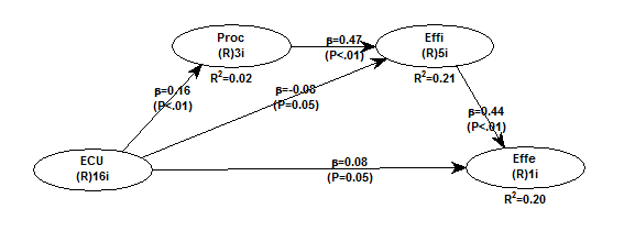
The graph below shows the expected values of Effe given Effi. The latter is one of the LVs that point at Effe in the model. The values of Effe and Effi are unstandardized.

Arguably a model with a dichotomous dependent variable cannot be viably tested with ordinary multiple regression because the dependent variable is not normally distributed (as it assumes only two values).
The graph below shows a histogram with the distribution of values of Effe. This variable's skewness is -0.423 and excess kurtosis is -1.821.

This is not a problem for WarpPLS because P values are calculated via nonparametric techniques that do not assume in their underlying design that any variables in the model meet parametric expectations; such as the expectations of univariate and multivariate unimodality and normality.
If a dependent variable refers to a probability (as in logistic regression), and is expected to be associated with a predictor according to a logistic function, you should use the Warp3 or Warp3 basic inner model algorithms to relate the two variables.
Model with endogenous dichotomous variable
There are two main ways in which a model with an endogenous dichotomous variable can be analyzed in PLS-SEM - via the logistic regression variables technique, and via the conditional probabilistic queries technique.
Logistic regression variables technique
Starting in version 8.0 of WarpPLS, the menu option “Explore logistic regression” allows you to create a logistic regression variable as a new indicator that has both unstandardized and standardized values. Logistic regression is normally used to convert an endogenous variable on a non-ratio scale (e.g., dichotomous) into a variable reflecting probabilities. You need to choose the variable to be converted, which should be an endogenous variable, and its predictors.
The new logistic regression variable is meant to be used as a replacement for the endogenous variable on which it is based. Two algorithms are available: probit and logit. The former is recommended for dichotomous variables; the latter for non-ratio variables where the number of different values (a.k.a. “distinct observations”) is greater than 2 but still significantly smaller than the sample size; e.g., 10 different values over a sample size of 100. The unstandardized values of a logistic regression variable are probabilities; going from 0 to 1.
Since a logistic regression variable can be severely collinear with its predictors, you can set a local full collinearity VIF cap for the logistic regression variable. Predictor-criterion collinearity, or lateral collinearity, is rarely assessed or controlled in classic logistic regression algorithms.
For more on this topic, see the links below.
Explore Logistic Regression in WarpPLS
Using Logistic Regression in PLS-SEM with Composites and Factors
Conditional probabilistic queries technique
How do we interpret the results of a model with an endogenous dichotomous variable, using the conditional probabilistic queries technique? Let us use the model below to illustrate the answer to this question. In this model we have one endogenous dichotomous variable “Success” that is significantly caused in a direct way by two predictors: “Projmgt” and “JSat”. The direct effect of a third predictor, namely "ECollab", is relatively small and borderline significant.

Let us assume that the unit of analysis is a team of people. The variable “Success” is coded as 0 or 1, meaning that a team is either successful or not. After standardization, the 0 and 1 will be converted into a negative and a positive number. The standardized version of the variable “Success” will have a mean of zero and a standard deviation of 1.
One way to interpret the results is the following. The probability that a team will be successful (i.e., that “Success” > 0) is significantly affected by increases in the variables “Projmgt” and “JSat”.
WarpPLS users are able, starting in version 6.0, to calculate conditional probabilities as shown below, without having to resort to transformations based on assumed underlying functions, such as those performed by logistic regression. In this screen shot, only latent variables are used, and they are all assumed to be standardized.

In the screen shot above, we can see that the probability that a team will be successful (i.e., that “Success” > 0), if “Projmgt” > 1 and “JSat” > 1, is 52.2 percent. Stated differently, if “Projmgt” and “JSat” are high (greater than 1 standard deviation above the mean), then the probability of success is slightly greater than chance.
A probability of 52.2 percent is not that high. The reason why it is not higher, in the context of the conditional probabilistic query above, is that we are not including the variable "ECollab" in the mix. Still, it does not seem like “Projmgt” and “JSat” being high are sufficient conditions for success, although they may be necessary conditions.
Consider a different set of conditional probabilities. If a team is successful (i.e., if “Success” > 0), what is the probability that “Projmgt” and “JSat” are low for that team. The answer, shown in the screen below, is 1.3 percent. That is a very low probability, suggesting that “Projmgt” and “JSat” matter as necessary but not sufficient elements for success.

These are among the conditional probabilistic queries that users are able to make starting in version 6.0 of WarpPLS. Bayes’ theorem is used to produce the answers to the queries.
Subscribe to:
Posts (Atom)
