Dichotomous variables

There are several ways in which a model with an endogenous dichotomous variable can be analyzed in PLS-SEM - via the logistic regression variables technique, without any additional treatment, and via the conditional probabilistic queries technique. Below we discuss the first two options.

Logistic regression variables technique

Starting in version 8.0 of WarpPLS, the menu option “Explore logistic regression” allows you to create a logistic regression variable as a new indicator that has both unstandardized and standardized values. Logistic regression is normally used to convert an endogenous variable on a non-ratio scale (e.g., dichotomous) into a variable reflecting probabilities. You need to choose the variable to be converted, which should be an endogenous variable, and its predictors. 

The new logistic regression variable is meant to be used as a replacement for the endogenous variable on which it is based. Two algorithms are available: probit and logit. The former is recommended for dichotomous variables; the latter for non-ratio variables where the number of different values (a.k.a. “distinct observations”) is greater than 2 but still significantly smaller than the sample size; e.g., 10 different values over a sample size of 100. The unstandardized values of a logistic regression variable are probabilities; going from 0 to 1. 

Since a logistic regression variable can be severely collinear with its predictors, you can set a local full collinearity VIF cap for the logistic regression variable. Predictor-criterion collinearity, or lateral collinearity, is rarely assessed or controlled in classic logistic regression algorithms. 

For more on this topic, see the links below.

Explore Logistic Regression in WarpPLS

https://youtu.be/PO65ySuhPW0

Using Logistic Regression in PLS-SEM with Composites and Factors

https://youtu.be/c9ySXN4NVus

Without any additional treatment

Models with dichotomous endogenous variables can also be tested with WarpPLS without any additional treatment, although this may lead to path coefficient suppression as well as other problems. Based on preliminary Monte Carlo simulations, the following combination of algorithm and P value calculation method seems to be the most advisable, if users want to analyze models with composite-based algorithms: PLS regression and stable.

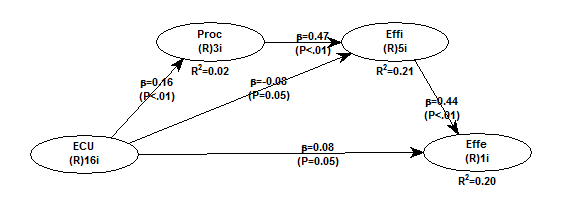
Below is a model with a dichotomous dependent variable - Effe. The variable assumes two values, 0 or 1, to reflect low or high levels of "effectiveness".

The graph below shows the expected values of Effe given Effi. The latter is one of the LVs that point at Effe in the model. The values of Effe and Effi are unstandardized.

Arguably a model with a dichotomous dependent variable cannot be viably tested with ordinary multiple regression because the dependent variable is not normally distributed (as it assumes only two values).

The graph below shows a histogram with the distribution of values of Effe. This variable's skewness is -0.423 and excess kurtosis is -1.821.

This is not a problem for WarpPLS because P values are calculated via nonparametric techniques that do not assume in their underlying design that any variables in the model meet parametric expectations; such as the expectations of univariate and multivariate unimodality and normality.

If a dependent variable refers to a probability (as in logistic regression), and is expected to be associated with a predictor according to a logistic function, you should use the Warp3 or Warp3 basic inner model algorithms to relate the two variables.

Model with endogenous dichotomous variable

There are two main ways in which a model with an endogenous dichotomous variable can be analyzed in PLS-SEM - via the logistic regression variables technique, and via the conditional probabilistic queries technique.

Logistic regression variables technique

Starting in version 8.0 of WarpPLS, the menu option “Explore logistic regression” allows you to create a logistic regression variable as a new indicator that has both unstandardized and standardized values. Logistic regression is normally used to convert an endogenous variable on a non-ratio scale (e.g., dichotomous) into a variable reflecting probabilities. You need to choose the variable to be converted, which should be an endogenous variable, and its predictors. 

The new logistic regression variable is meant to be used as a replacement for the endogenous variable on which it is based. Two algorithms are available: probit and logit. The former is recommended for dichotomous variables; the latter for non-ratio variables where the number of different values (a.k.a. “distinct observations”) is greater than 2 but still significantly smaller than the sample size; e.g., 10 different values over a sample size of 100. The unstandardized values of a logistic regression variable are probabilities; going from 0 to 1. 

Since a logistic regression variable can be severely collinear with its predictors, you can set a local full collinearity VIF cap for the logistic regression variable. Predictor-criterion collinearity, or lateral collinearity, is rarely assessed or controlled in classic logistic regression algorithms. 

For more on this topic, see the links below.

Explore Logistic Regression in WarpPLS

https://youtu.be/PO65ySuhPW0

Using Logistic Regression in PLS-SEM with Composites and Factors

https://youtu.be/c9ySXN4NVus

Conditional probabilistic queries technique

How do we interpret the results of a model with an endogenous dichotomous variable, using the conditional probabilistic queries technique? Let us use the model below to illustrate the answer to this question. In this model we have one endogenous dichotomous variable “Success” that is significantly caused in a direct way by two predictors: “Projmgt” and “JSat”. The direct effect of a third predictor, namely "ECollab", is relatively small and borderline significant.

Let us assume that the unit of analysis is a team of people. The variable “Success” is coded as 0 or 1, meaning that a team is either successful or not. After standardization, the 0 and 1 will be converted into a negative and a positive number. The standardized version of the variable “Success” will have a mean of zero and a standard deviation of 1.

One way to interpret the results is the following. The probability that a team will be successful (i.e., that “Success” > 0) is significantly affected by increases in the variables “Projmgt” and “JSat”.

WarpPLS users are able, starting in version 6.0, to calculate conditional probabilities as shown below, without having to resort to transformations based on assumed underlying functions, such as those performed by logistic regression. In this screen shot, only latent variables are used, and they are all assumed to be standardized.

In the screen shot above, we can see that the probability that a team will be successful (i.e., that “Success” > 0), if “Projmgt” > 1 and “JSat” > 1, is 52.2 percent. Stated differently, if “Projmgt” and “JSat” are high (greater than 1 standard deviation above the mean), then the probability of success is slightly greater than chance.

A probability of 52.2 percent is not that high. The reason why it is not higher, in the context of the conditional probabilistic query above, is that we are not including the variable "ECollab" in the mix. Still, it does not seem like “Projmgt” and “JSat” being high are sufficient conditions for success, although they may be necessary conditions.

Consider a different set of conditional probabilities. If a team is successful (i.e., if “Success” > 0), what is the probability that “Projmgt” and “JSat” are low for that team. The answer, shown in the screen below, is 1.3 percent. That is a very low probability, suggesting that “Projmgt” and “JSat” matter as necessary but not sufficient elements for success.

These are among the conditional probabilistic queries that users are able to make starting in version 6.0 of WarpPLS. Bayes’ theorem is used to produce the answers to the queries.

WarpPLS 8.0 upgraded to stable: Logistic regression, full latent growth graphs, HTMT2 ratios, and more!

Dear colleagues:

Version 8.0 of WarpPLS is now available as a stable version. You can download and install it for a free trial from:

https://warppls.com

Each new version of the software incorporates features that aim at achieving an important end goal: to allow users to employ SEM to conduct any of the major statistical tests; from relatively simple tests such as comparisons of means, to more sophisticated ones such as nonlinear SEM tests employing logistic regression. Among the community of users of this software, there are very sophisticated SEM experts that constantly challenge us to implement new data analysis features, as well as to make the existing features as easy to use as possible. Because of the constant input from our users, including those who are very knowledgeable about SEM, the software now arguably provides the most extensive set of features of any SEM software. We hope to continue in this path as the SEM field evolves. Below we outline new features added to the current version of the software.

Logistic regression variables. The menu option “Explore logistic regression” now allows you to create a logistic regression variable as a new indicator that has both unstandardized and standardized values. Logistic regression is normally used to convert an endogenous variable on a non-ratio scale (e.g., dichotomous) into a variable reflecting probabilities. You need to choose the variable to be converted, which should be an endogenous variable, and its predictors. The new logistic regression variable is meant to be used as a replacement for the endogenous variable on which it is based. Two algorithms are available: probit and logit. The former is recommended for dichotomous variables; the latter for non-ratio variables where the number of different values (a.k.a. “distinct observations”) is greater than 2 but still significantly smaller than the sample size; e.g., 10 different values over a sample size of 100. The unstandardized values of a logistic regression variable are probabilities; going from 0 to 1. Since a logistic regression variable can be severely collinear with its predictors, you can set a local full collinearity VIF cap for the logistic regression variable. Predictor-criterion collinearity, or lateral collinearity (Kock & Lynn, 2012), is rarely assessed or controlled in classic logistic regression algorithms.

Absolute and relative variation measures. You can now view the number of different values (a.k.a. “distinct observations”) for all indicators and latent variables, as well as the ratio between the number of different values and sample size. The first is an absolute and the second a relative variation measure. These are available under the menu options “View or save correlations and descriptive statistics for indicators” and “View latent variable coefficients”, respectively. These measures can help inform decisions about whether to use logistic regression, particularly in connection with endogenous latent variables. If the number of different values is significantly smaller than the sample size (e.g., 10 different values over a sample size of 100) for an endogenous latent variable, that means that a new logistic regression variable could be created and used as a replacement for the endogenous variable. If several predictors are available, the new logistic regression variable will incorporate more variation than the endogenous variable on which it is based, which will typically be reflected in larger coefficients of association (e.g., path coefficients) when the logistic regression variable is used in the model.

Graphs for full latent growth coefficients. You can now view several graphs for each of the full latent growth coefficients provided under the menu option “Explore full latent growth”. Full latent growth coefficients have a number of applications, such as: moderating effects analyses, nonlinearity tests, multi-group and measurement invariance tests, and the assessment of moderated mediation effects. Each of the graphs is made up of several plots, which refer to changes in the coefficients selected (e.g., path coefficients) for the relationship between the variables shown in the X and Y axes, as the latent growth variable goes from low to high. The following graph menu options are available: “Full sample splits (megaphones)”, “Partial sub-samples splits (megaphones)”, “Full sample splits (bars)”, “Partial sub-samples splits (bars)”, “Full sample splits (lines)”, and “Partial sub-samples splits (lines)”.

HTMT2 ratios. The sub-option “'Discriminant validity coefficients (extended set)”, under the menu option “Explore additional coefficients and indices”, now allows you to inspect the newest version of the set of heterotrait-monotrait (HTMT) ratios calculated by the software. These have been dubbed HTMT2 ratios. The HTMT and HTMT2 ratios have been proposed for discriminant validity assessment, particularly in the context of composite-based SEM via classic PLS algorithms; as opposed to factor-based SEM via modern algorithms that estimate factors (which have been available from this software for quite some time now). Discriminant validity is a measure of the quality of a measurement instrument; the instrument itself is typically a set of question-statements. A measurement instrument has good discriminant validity if the question-statements (or other measures) associated with each latent variable are not confused by the respondents, in terms of their meaning, with the question-statements associated with other latent variables.

Incremental interface improvement. This is conducted in each new version of the software. At several points the code has been modified so that the user interface experiences are improved. This has led in several cases to what appears to be a smoother flow through the several steps and procedures guided by the user interface. Several elements of the graphical user interface, such as screens and warning messages, have been optimized so that users can perform SEM analysis tasks with only a few clicks – and in a straightforward fashion. Nevertheless, care is always taken to ensure that the user interfaces do not change too much, otherwise users would have to re-learn how to use the interface whenever a new version is released.

Incremental code optimization. This is also conducted in each new version of the software. At several points the code has been optimized for speed, stability, and coefficient estimation precision. In some cases, the optimization has led to lesser propagation of sampling error, making the software reach accurate results at lower sample sizes – that is, increasing the statistical efficiency of the software. These incremental code optimization changes have led to incremental gains in speed even as new features have been added. More often than not, new features require additional computational steps and often complex calculations, mostly to generate internal checks and coefficients that were not available before.

Take a look at the following videos, which have been created using this new version. They illustrate the new features outlined above.

Explore Logistic Regression in WarpPLS

View the Number of Different Values for Variables in WarpPLS

View Full Latent Growth Graphs in WarpPLS

Holistic Measurement Model Assessment in SEM with WarpPLS

Reduce Common Structural Variation with WarpPLS

Assessing Multiple Reciprocal Relationships in SEM with WarpPLS

Choose the Correlation Signs for Anchor Variables in a Multilevel Analysis with WarpPLS

Using Logistic Regression in PLS-SEM with Composites and Factors

Conducting a What-if Analysis in PLS-SEM with Analytic Composites

Reference:

Kock, N., & Lynn, G. (2012). Lateral collinearity and misleading results in variance-based SEM: An illustration and recommendations. Journal of the Association for Information Systems, 13(7), 546-580.

Best regards to all!

WarpPLS 8.0 beta now available: Logistic regression, full latent growth graphs, HTMT2 ratios, and more!

Dear colleagues:

Version 8.0 of WarpPLS is now available, as a beta version. You can download and install it for a free trial from:

https://warppls.com

Each new version of the software incorporates features that aim at achieving an important end goal: to allow users to employ SEM to conduct any of the major statistical tests; from relatively simple tests such as comparisons of means, to more sophisticated ones such as nonlinear SEM tests employing logistic regression. Among the community of users of this software, there are very sophisticated SEM experts that constantly challenge us to implement new data analysis features, as well as to make the existing features as easy to use as possible. Because of the constant input from our users, including those who are very knowledgeable about SEM, the software now arguably provides the most extensive set of features of any SEM software. We hope to continue in this path as the SEM field evolves. Below we outline new features added to the current version of the software.

Logistic regression variables. The menu option “Explore logistic regression” now allows you to create a logistic regression variable as a new indicator that has both unstandardized and standardized values. Logistic regression is normally used to convert an endogenous variable on a non-ratio scale (e.g., dichotomous) into a variable reflecting probabilities. You need to choose the variable to be converted, which should be an endogenous variable, and its predictors. The new logistic regression variable is meant to be used as a replacement for the endogenous variable on which it is based. Two algorithms are available: probit and logit. The former is recommended for dichotomous variables; the latter for non-ratio variables where the number of different values (a.k.a. “distinct observations”) is greater than 2 but still significantly smaller than the sample size; e.g., 10 different values over a sample size of 100. The unstandardized values of a logistic regression variable are probabilities; going from 0 to 1. Since a logistic regression variable can be severely collinear with its predictors, you can set a local full collinearity VIF cap for the logistic regression variable. Predictor-criterion collinearity, or lateral collinearity (Kock & Lynn, 2012), is rarely assessed or controlled in classic logistic regression algorithms.

Absolute and relative variation measures. You can now view the number of different values (a.k.a. “distinct observations”) for all indicators and latent variables, as well as the ratio between the number of different values and sample size. The first is an absolute and the second a relative variation measure. These are available under the menu options “View or save correlations and descriptive statistics for indicators” and “View latent variable coefficients”, respectively. These measures can help inform decisions about whether to use logistic regression, particularly in connection with endogenous latent variables. If the number of different values is significantly smaller than the sample size (e.g., 10 different values over a sample size of 100) for an endogenous latent variable, that means that a new logistic regression variable could be created and used as a replacement for the endogenous variable. If several predictors are available, the new logistic regression variable will incorporate more variation than the endogenous variable on which it is based, which will typically be reflected in larger coefficients of association (e.g., path coefficients) when the logistic regression variable is used in the model.

Graphs for full latent growth coefficients. You can now view several graphs for each of the full latent growth coefficients provided under the menu option “Explore full latent growth”. Full latent growth coefficients have a number of applications, such as: moderating effects analyses, nonlinearity tests, multi-group and measurement invariance tests, and the assessment of moderated mediation effects. Each of the graphs is made up of several plots, which refer to changes in the coefficients selected (e.g., path coefficients) for the relationship between the variables shown in the X and Y axes, as the latent growth variable goes from low to high. The following graph menu options are available: “Full sample splits (megaphones)”, “Partial sub-samples splits (megaphones)”, “Full sample splits (bars)”, “Partial sub-samples splits (bars)”, “Full sample splits (lines)”, and “Partial sub-samples splits (lines)”.

HTMT2 ratios. The sub-option “'Discriminant validity coefficients (extended set)”, under the menu option “Explore additional coefficients and indices”, now allows you to inspect the newest version of the set of heterotrait-monotrait (HTMT) ratios calculated by the software. These have been dubbed HTMT2 ratios. The HTMT and HTMT2 ratios have been proposed for discriminant validity assessment, particularly in the context of composite-based SEM via classic PLS algorithms; as opposed to factor-based SEM via modern algorithms that estimate factors (which have been available from this software for quite some time now). Discriminant validity is a measure of the quality of a measurement instrument; the instrument itself is typically a set of question-statements. A measurement instrument has good discriminant validity if the question-statements (or other measures) associated with each latent variable are not confused by the respondents, in terms of their meaning, with the question-statements associated with other latent variables.

Incremental interface improvement. This is conducted in each new version of the software. At several points the code has been modified so that the user interface experiences are improved. This has led in several cases to what appears to be a smoother flow through the several steps and procedures guided by the user interface. Several elements of the graphical user interface, such as screens and warning messages, have been optimized so that users can perform SEM analysis tasks with only a few clicks – and in a straightforward fashion. Nevertheless, care is always taken to ensure that the user interfaces do not change too much, otherwise users would have to re-learn how to use the interface whenever a new version is released.

Incremental code optimization. This is also conducted in each new version of the software. At several points the code has been optimized for speed, stability, and coefficient estimation precision. In some cases, the optimization has led to lesser propagation of sampling error, making the software reach accurate results at lower sample sizes – that is, increasing the statistical efficiency of the software. These incremental code optimization changes have led to incremental gains in speed even as new features have been added. More often than not, new features require additional computational steps and often complex calculations, mostly to generate internal checks and coefficients that were not available before.

Take a look at the following videos, which have been created using this new version. They illustrate the new features outlined above.

Explore Logistic Regression in WarpPLS

View the Number of Different Values for Variables in WarpPLS

View Full Latent Growth Graphs in WarpPLS

Holistic Measurement Model Assessment in SEM with WarpPLS

Reduce Common Structural Variation with WarpPLS

Assessing Multiple Reciprocal Relationships in SEM with WarpPLS

Choose the Correlation Signs for Anchor Variables in a Multilevel Analysis with WarpPLS

Using Logistic Regression in PLS-SEM with Composites and Factors

Conducting a What-if Analysis in PLS-SEM with Analytic Composites

Reference:

Kock, N., & Lynn, G. (2012). Lateral collinearity and misleading results in variance-based SEM: An illustration and recommendations. Journal of the Association for Information Systems, 13(7), 546-580.

Best regards to all!