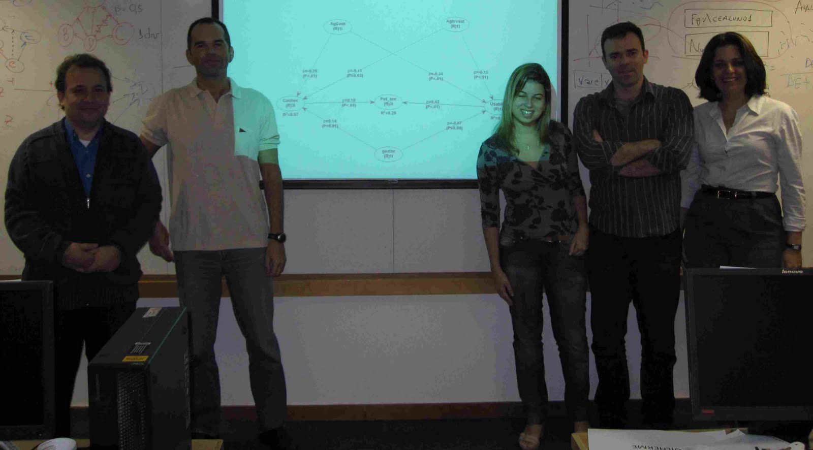
Below are some photos from the June 2011 WarpPLS workshop at Fundação Getúlio Vargas, one of the highest ranked and most prestigious universities in Brazil in its main areas of focus. FGV’s main foci are business management and public administration. The workshop was in Rio de Janeiro. The workshop participants included faculty, doctoral students, and masters’ students at FGV.
This was a very hands-on workshop, as the participants had taken a course in structural equation modeling prior to it. They used Amos in that course, which was great because the workshop then highlighted the power of WarpPLS vis-à-vis a well established and also very useful tool for multivariate analyses with latent variables (Amos). We had about 15 contact hours for this workshop. Activities included commentaries based on video clips, live demonstrations, discussions of selected readings, and practical assignments focusing on linear and nonlinear empirical data analyses.
About 30 percent of the workshop was set aside for “free data analyses”, building on data that the participants brought into the workshop. That is, the participants had time to analyze their own data, and solve specific problems with my help. (There are always issues that are specific to a given dataset; e.g., problems with indicator loadings and interpretation of nonlinear results.) There was also a team workshop project, where participant teams presented an independent empirical study with analyses employing WarpPLS.
Some of the participants were faculty members from other universities in Rio de Janeiro, as well as employees of a few major research and training organizations in Brazil. Among these organizations were Fundação Oswaldo Cruz (a.k.a. FIOCRUZ), and the Escola de Comando e Estado Maior do Exército (ECEME). FIOCRUZ is one of the world’s foremost public health organizations, known for its strengths in various related areas, including epidemiological research. ECEME is an education institution that prepares officers of the Brazilian Army to take up command positions at the rank of General.
Monday, July 18, 2011
Tuesday, June 28, 2011
WarpPLS’ treatment of formative latent variables: PLS regression is more conservative and stable
For a more detailed discussion of the issues addressed in this post, please see the publication below.
Kock, N., & Mayfield, M. (2015). PLS-based SEM algorithms: The good neighbor assumption, collinearity, and nonlinearity. Information Management and Business Review, 7(2), 113-130.
***
WarpPLS implements a number of composite-based and factor-based algorithms. One of the composite-based algorithms is often referred to as Wold’s original “PLS regression” algorithm to calculate indicator weights, for both formative and reflective variables. PLS regression was developed by Wold, and is slightly different from the modified versions often referred to as modes A and B, which are the ones normally used in other publicly available PLS-based structural equation modeling software. These modified versions implement an underlying algorithmic assumption that Lohmöller called the "good neighbor" assumption, whereby weights are influenced by inner model links.
Generally speaking, the PLS regression algorithm generates coefficients that are more stable and robust – i.e., reliable for hypothesis testing. It also tends to minimize collinearity. On the other hand, it may be lead to a higher demand for computational power in some cases, which may be the reason why modified versions have been implemented. Lohmöller discusses multiple algorithm versions, with some characteristics placing them within broad types called “modes” – see Lohmöller (1989), the PLS "bible", for more details. Personal computers were not that powerful in the 1980s.
Moreover, the type of nonlinear treatment employed by WarpPLS is difficult to perform with Lohmöller’s underlying algorithm (the "good neighbor" assumption), whereby the outer model is influenced by the inner model. The problem is that with Lohmöller’s algorithm, as a model changes, the weights and loadings also change, even if the latent variables do not change. That is, with Lohmöller’s algorithm, two models with the same latent variables but different structures (i.e., links among latent variables) will have different weights and loadings.
The weights of formative latent variables will be essentially the same in WarpPLS as they would be if the variables were defined as reflective. That is, they will be obtained by an iterative algorithm that stops when two conditions are met: (a) the weights between indicators and latent variable are standardized partial regression coefficients calculated with the indicators as independent variables and the latent variable as the dependent variable; and (b) the regression equation expressing the latent variable as a combination of the indicators has an error term of zero.
So why should the user define a latent variable as formative or reflective? The reason are the interpretations of the outputs generated by the software. When a latent variable is formative, both the P values for the weights and the variance inflation factors for the indicators should be generally low; ideally below 0.05 and 2.5, respectively.
True formative variables are fundamentally different from true reflective variables; there are cases that can be seen as “in between” formative and reflective. True formative and reflective variables behave differently, whether the software treats them differently or not. For example, with true formative variables you would expect indicators to be significantly associated with the scores of their respective latent variable; which is indicated by low P values for their weights. However, you would not normally expect the indicators to be redundant; which is indicated by low variance inflation factors for the indicators.
The way formative variables are treated in Lohmöller’s approach leads to unstable weights, with the signs of weights frequently changing in the resample set. See Temme et al. (2006) for a discussion on this phenomenon. Lohmöller’s approach also leads to “lateral” collinearity; or collinearity between predictor and criteria latent variables. This “stealth” type of collinearity often leads to inflated path coefficients for links involving formative latent variables.
Formative variables don't "become reflective", or vice-versa, if one or another algorithm is used. This is a common misconception among users of PLS-based SEM software.
References
Kock, N., & Mayfield, M. (2015). PLS-based SEM algorithms: The good neighbor assumption, collinearity, and nonlinearity. Information Management and Business Review, 7(2), 113-130.
Lohmöller, J.-B. (1989). Latent variable path modeling with partial least squares. Heidelberg, Germany: Physica-Verlag.
Temme, D., Kreis, H., & Hildebrandt, L. (2006). PLS path modeling – A software review. Berlin, Germany: Institute of Marketing, Humboldt University Berlin.
Labels:
formative,
Lohmöller,
PLS regression,
reflective,
warppls,
Wold
Saturday, June 25, 2011
Dealing with country-specific number punctuation systems
WarpPLS users in countries that adopt number punctuation systems different from that adopted in the USA may have problems when using Excel to manipulate WarpPLS files.
For instance, in Brazil a comma is used to separate the integer from the fractional part of a real number (e.g., 1,431), whereas in the USA a period is used for that purpose (e.g., 1.431).
Because of that, a coefficient calculated by WarpPLS and exported into a .txt file as “1.431” may be read by a Brazilian version of Excel as one thousand four hundred and thirty-one, and not as one plus the 431/1000 fraction.
This tends to happen in certain types of analyses, such as second order latent variable analyses, where WarpPLS outputs are used as inputs after manipulation with country-specific versions of Excel.
A simple way to solve this problem is to use Excel, Notepad, or another simple text editing tool and replace the offending punctuation items, all points with commas (or vice-versa) for example, before using the inputs for other purposes.
Saturday, June 18, 2011
Testing the significance of mediating effects with WarpPLS using the Preacher & Hayes approach
This post refers to the use of WarpPLS to test a mediating effect using what is often referred to as the Preacher and Hayes approach. This approach employs the Sobel's standard error method (for a recent discussion, see: Kock, 2013). You can also test mediating effects directly with WarpPLS, using indirect and total effect outputs:
http://warppls.blogspot.com/2013/04/testing-mediating-effects-directly-with.html
Previously I also discussed on this blog the classic approach proposed by Baron & Kenny (1986) to test the significance of mediating effects with WarpPLS.
An approach that is an alternative to Baron & Kenny's (1986) approach has been proposed by Preacher & Hayes (2004) to test the significance of mediating effects. This approach has been further extended by Hayes & Preacher (2010) for nonlinear relationships.
These approaches are implemented through an Excel spreadsheet available from the “Resources” area of the WarpPLS.com site, under “Excel files”. The spreadsheet, which implements the Sobel's standard error method, can be used with coefficients generated based on linear and nonlinear analyses.
The Excel spreadsheet above takes as inputs coefficients generated by WarpPLS, including path coefficients and their standard errors. The formulas used in it are discussed in a recent publication (Kock, 2014). The outputs are Sobel’s standard errors, product path coefficients, as well as T and P values, for mediating effects.
References
Baron, R.M., & Kenny, D.A. (1986). The moderator–mediator variable distinction in social psychological research: Conceptual, strategic, and statistical considerations. Journal of Personality & Social Psychology, 51(6), 1173-1182.
Hayes, A.F., & Preacher, K.J. (2010). Quantifying and testing indirect effects in simple mediation models when the constituent paths are nonlinear. Multivariate Behavioral Research, 45(4), 627-660.
Kock, N. (2014). Advanced mediating effects tests, multi-group analyses, and measurement model assessments in PLS-based SEM. International Journal of e-Collaboration, 10(3), 1-13.
(http://www.scriptwarp.com/warppls/pubs/Kock_2014_UseSEsESsLoadsWeightsSEM.pdf)
Preacher, K.J., & Hayes, A.F. (2004). SPSS and SAS procedures for estimating indirect effects in simple mediation models. Behavior Research Methods, Instruments, & Computers, 36 (4), 717-731.
Multi-group analysis with WarpPLS: Comparing path coefficients for two or more group samples
Starting in version 6.0 of WarpPLS, the menu options “Explore multi-group analyses” and “Explore measurement invariance” allow you to conduct analyses where the data is segmented in various groups, all possible combinations of pairs of groups are generated, and each pair of groups is compared. In multi-group analyses normally path coefficients are compared, whereas in measurement invariance assessment the foci of comparison are loadings and/or weights. The grouping variables can be unstandardized indicators, standardized indicators, and labels. These types of analyzes can also be conducted via the new menu option “Explore full latent growth”, which presents several advantages (as discussed in the WarpPLS User Manual).
Related YouTube videos:
Explore Multi-Group Analyses in WarpPLS
Explore Measurement Invariance in WarpPLS
The text below is for an older version of this post. It discusses other approaches to multi-group analysis that are only partially automated, and that are thus more time-consuming to implement.
***
I previously discussed on this post multi-group analysis with WarpPLS from the perspective of comparing means of two or more groups. This is also explored in an article titled: Using WarpPLS in e-collaboration studies: What if I have only one group and one condition?
A different type of multi-group analysis would be one in which the same model is analyzed for two or more different samples, where each sample refers to a data group.
For example, a researcher could test the same model with data from the USA and Mexico. In this case, two project files would be used, and the goal of the multi-group analysis would be to assess whether the path coefficients differ significantly across groups.
An approach to conduct this type of multi-group analysis, employing the pooled and Satterthwaite standard error methods, is discussed in a recent publication (Kock, 2014). This approach is implemented through an Excel spreadsheet available from the “Resources” area of the WarpPLS.com site, under “Excel files”.
The Excel spreadsheet above takes as inputs coefficients generated by WarpPLS, including path coefficients and their standard errors. The outputs are T and P values for each pair of coefficients being compared. The formulas used in it are discussed in a recent publication (Kock, 2014).
Reference
Kock, N. (2014). Advanced mediating effects tests, multi-group analyses, and measurement model assessments in PLS-based SEM. International Journal of e-Collaboration, 10(3), 1-13.
Labels:
group samples,
multi-group analysis,
P value,
path coefficient,
warppls
Friday, April 22, 2011
Using WarpPLS in E-Collaboration Studies: Descriptive Statistics, Settings, and Key Analysis Results
A new article discussing WarpPLS is available. The article is titled “Using WarpPLS in E-Collaboration Studies: Descriptive Statistics, Settings, and Key Analysis Results”. It has been recently published in the International Journal of e-Collaboration. A full text version of the article is available here as a PDF file. Below is the abstract of the article.
This is a follow-up on a previous article (Kock, 2010b) discussing the five main steps through which a nonlinear structural equation modeling analysis could be conducted with the software WarpPLS (warppls.com). Both this and the previous article use data from the same e-collaboration study as a basis for the discussion of important WarpPLS features. Unlike in the previous article, the focus here is on specific features related to saving and analyzing grouped descriptive statistics, viewing and changing analysis algorithm and resampling settings, and viewing and saving the various minor and major results of the analysis. Even though its focus is on an e-collaboration study this article contributes to the broad literature on multivariate analysis methods, in addition to the more specific research literature on e-collaboration. The reason for this is that the vast majority of relationships between variables, in investigations of both natural and behavioral phenomena, are nonlinear; usually taking the form of U and S curves. Structural equation modeling software tools, whether variance- or covariance-based, typically do not estimate coefficients of association based on nonlinear analysis algorithms. WarpPLS is an exception in this respect. Without taking nonlinearity into consideration, the results can be misleading; especially in complex and multi-factorial situations such as those stemming from e-collaboration in virtual teams.
Wednesday, April 20, 2011
Transitioning from WarpPLS 1.0 to 2.0
Transitioning from version 1.0 to 2.0 of WarpPLS is very easy. Even though both can be installed and ran on the same computer, and should not interfere with each other, I recommend using only the latest version.
There is no need to uninstall version 1.0, but if you want to do so you can follow the instructions at the beginning of the User Manual for version 1.0.
Version 1.0 users can enter the same license information as for version 1.0; it will work for version 2.0 for the remainder of their license periods.
Project files generated with version 1.0 can be used with version 2.0, but only after running Step 5 again. This is needed because version 2.0 generates additional estimates.
Enjoy!
There is no need to uninstall version 1.0, but if you want to do so you can follow the instructions at the beginning of the User Manual for version 1.0.
Version 1.0 users can enter the same license information as for version 1.0; it will work for version 2.0 for the remainder of their license periods.
Project files generated with version 1.0 can be used with version 2.0, but only after running Step 5 again. This is needed because version 2.0 generates additional estimates.
Enjoy!
Subscribe to:
Posts (Atom)