Full latent growth and its use in PLS-SEM: Testing moderating relationships

The article below explains how one can conduct a full latent growth analysis, in the context of structural equation modeling via partial least squares (PLS-SEM). This type of analysis can be viewed as a comprehensive analysis of moderating effects where the moderating variable is “latent”, not “disrupting” the model in any way.

Kock (2020). Full latent growth and its use in PLS-SEM: Testing moderating relationships. Data Analysis Perspectives Journal, 1(1), 1-5.

A link to a PDF file is available ().

Abstract:

A full latent growth analysis, in the context of structural equation modeling via partial least squares (PLS-SEM), can be viewed as a comprehensive analysis of moderating effects where the moderating variable is “latent”, not “disrupting” the model in any way. In this paper we illustrate such an analysis employing WarpPLS, a leading PLS-SEM software tool.

New PLS-based SEM email distribution list

A new email distribution list is available for those who share a common interest in partial least squares (PLS) regression and its use in structural equation modeling (SEM). To check it out click here.

There is no need for two-way arrows in WarpPLS

In covariance-based structural equation modeling (SEM) software tools, often one has to explicitly model correlations between predictor latent variables (LVs) to obtain related estimates. In WarpPLS, correlations between predictor LVs are automatically taken into consideration in the calculation of path coefficients.

It should be noted that when we say "two-way arrows" we are not referring to reciprocal relationships. Reciprocal relationships are usually represented via two straight arrows, each arrow pointing in a different direction. What we call "two-way arrows" here are representations of correlations.

The path coefficients calculated by WarpPLS are true standardized partial regression coefficients, of the same type as those calculated through multiple regression analysis. The difference is, of course, that in WarpPLS the model variables are LVs, which are usually measured through more than one indicator. With multiple regression, only one measure (or indicator) is used for each variable in the model.

Naming of latent variable indicators in WarpPLS

The indicator names are the headings of your raw data file, which are also shown on a few software screens during Step 2. That is the step where you read the raw data used in the SEM analysis. The indicator names are displayed at the top of the table on the figure below, a screen from Step 3; click on it to enlarge.

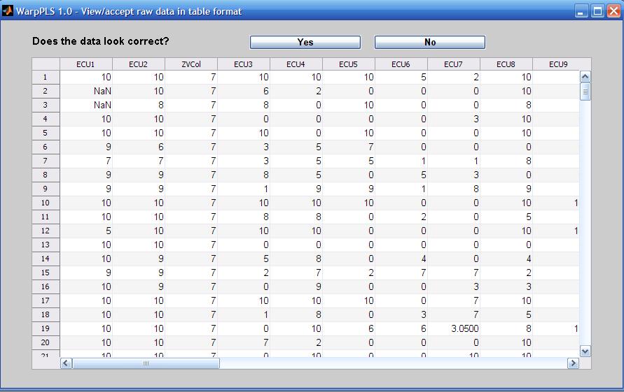
The software does not force users to restrict the names of indicators to a set number of characters (e.g., seven), or to exclude certain types of characters (e.g., blank spaces) from them. Nevertheless, it is usually a good idea to follow a few simple rules when naming indicators:

- Make the indicator names 7 characters in length, or less. This will ensure that they will not take up too much space on various screens and reports. In fact, in reports saved in text files, any character after the seventh is removed by the software. Otherwise the text file will become difficult to read without manual editing.

- Name the indicators using their latent variable name as a reference, and using sequential numbers at the end. For example, indicators that refer to the latent variable “ECU” should be named: “ECU1”, “ECU2”, “ECU3”, and so on.

- Do not use blank spaces in the indicator names. If you do, and an indicator name is long, the software may show the indicator split on two different rows on the model screen (Step 4), when you choose to show indicators on the model.

Field studies, small samples, and WarpPLS

Let us assume that a researcher wants to evaluate the effectiveness of new management method by conducting an intervention study in one single organization.

In this example, the researcher facilitates the use of a new management method by 20 managers in the organization, and then measures their degree of adoption of the method and their effectiveness.

The above is an example of a field study. Often field studies will yield small datasets, which will not conform to parametric analysis (e.g., ANOVA and ordinary multiple regression) pre-conditions. For example, the data will not typically be normally distributed.

WarpPLS can be very useful in the analysis of this type of data.

One reason is that, with small sample sizes, it may be difficult to identify linear relationships that are strong enough to be statistically significant (at P lower than 0.05, or less). Since WarpPLS implements nonlinear analysis algorithms, it can be very useful in the analysis of small samples.

Another reason is that P values are calculated through resampling, a nonparametric approach to statistical significance estimation. For small samples (i.e., lower than 100), jackknifing is the recommended resampling approach. Bootstrapping is recommended only for sample sizes greater than 100.

Geographically distributed collaborative SEM analysis using WarpPLS

I am currently conducting a geographically distributed collaborative SEM analysis using WarpPLS. The analysis involves a few people in different states of the USA, and two people outside the country. The collaborators are not only separated by large distances, but also operate in different time zones.

Yet, we have no problems collaborating. The collaboration is asynchronous – one person does some work one day, and shares it with the others, who review the work in the next few days and respond.

Since we all have WarpPLS installed on our computers, we exchange different versions of a WarpPLS project file (extension “.prj”) with the same dataset. This way we can do analyses in turns, and discuss the results on emails.

Each slightly different project file is saved with a different name – e.g., W3J_InfoOvld_2010_03_02.prj, W3B_InfoOvld_2010_03_02.prj, W2J_InfoOvld_2010_03_02.prj etc.

In the examples above, the first three letters indicate the SEM algorithm used (W3 = Warp3 PLS Regression; W2 = Warp2 PLS Regression), and the resampling method used (J = jackknifing; B = bootstrapping). The second part of the name describes the dataset, and the final part the date.

This is just one way of naming files. It works for our particular project, but more elaborate file names can be used in more complex collaborative SEM analyses.

This geographically distributed collaborative SEM analysis highlights one of the advantages of WarpPLS over other SEM software: all that is needed for the analysis is contained in one single project file.

Moreover, the project file will typically be only a few hundred kilobytes in size. In spite of its small size, the file includes the original data, and all of the results of the analysis.

One member of our team asked me how the project file can be so small. The reason is that all of the SEM analysis results are stored in a format that allows for their rendering every time they are viewed.

Plots of nonlinear relationships, for example, are not stored as bitmaps, but as equations that allow WarpPLS  to re-create those plots at the time of viewing.

What are the inner and outer models in SEM?

In a structural equation modeling (SEM) analysis, the inner model is the part of the model that describes the relationships among the latent variables that make up the model. The outer model is the part of the model that describes the relationships among the latent variables and their indicators.

In this sense, the path coefficients are inner model parameter estimates. The weights and loadings are outer model parameter estimates. The inner and outer models are also frequently referred to as the structural and measurement models, respectively.

More precisely, the mathematical equations that express the relationships among latent variables are referred to as the structural model. The equations that express the relationships among latent variables and indicators are referred to as the measurement model.

The term structural equation model is used to refer to both the structural and measurement model, combined.

Nonlinearity and type I and II errors in SEM analysis

Many relationships between variables studied in the natural and behavioral sciences seem to be nonlinear, often following a J-curve pattern (a.k.a. U-curve pattern). Other common relationships include the logarithmic, hyperbolic decay, exponential decay, and exponential. These and other relationships are modeled by WarpPLS.

Yet, the vast majority of statistical analysis methods used in the natural and behavioral sciences, from simple correlation analysis to structural equation modeling, assume relationships to be linear in the estimation of coefficients of association (e.g., Pearson correlations, standardized partial regression coefficients).

This may significantly distort results, especially in multivariate analyses, increasing the likelihood that researchers will commit type I and II errors in the same study. A type I error occurs in SEM analysis when an insignificant (the technical term is "non-significant") association is estimated as being significant (i.e., a “false positive”); a type II error occurs when a significant association is estimated as being insignificant (i.e., an existing association is “missed”).

The figure below shows a distribution of points typical of a J-curve pattern involving two variables, disrupted by uncorrelated error. The pattern, however, is modeled as a linear relationship. The line passing through the points is the best linear approximation of the distribution of points. It yields a correlation coefficient of .582. In this situation, the variable on the horizontal axis explains 33.9 percent of the variance of the variable on the vertical axis.

The figure below shows the same J-curve scatter plot pattern, but this time modeled as a nonlinear relationship. The curve passing through the points is the best nonlinear approximation of the distribution of the underlying J-curve, and excludes the uncorrelated error. That is, the curve does not attempt to model the uncorrelated error, only the underlying nonlinear relationship. It yields a correlation coefficient of .983. Here the variable on the horizontal axis explains 96.7 percent of the variance of the variable on the vertical axis.

WarpPLS transforms (or “warps”) J-curve relationship patterns like the one above BEFORE the corresponding path coefficients between each pair of variables are calculated. It does the same for many other nonlinear relationship patterns. In multivariate analyses, this may significantly change the values of the path coefficients, reducing the risk that researchers will commit type I and II errors.

The risk of committing type I and II errors is particularly high when: (a) a block of latent variables includes multiple predictor variables pointing and the same criterion variable; (b) one or more relationships between latent variables are significantly nonlinear; and (c) the predictor latent variables are correlated, even if they clearly measure different constructs (suggested by low variance inflation factors).

How do I control for the effects of one or more demographic variables in an SEM analysis?

As part of an SEM analysis using WarpPLS, a researcher may want to control for the effects of one ore more variables. This is typically the case with what are called “demographic variables”, or variables that measure attributes of a given unit of analysis that are (usually) not expected to influence the results of the SEM analysis.

For example, let us assume that one wants to assess the effect of a technology, whose intensity of use is measured by a latent variable T, on a behavioral variable measured by B. The unit of analysis for B is the individual user; that is, each row in the dataset refers to an individual user of the technology. The researcher hypothesizes that the association between T and B is significant, so a direct link between T and B is included in the model.

If the researcher wants to control for age (A) and gender (G), which have also been collected for each individual, in relation to B, all that is needed is to include the variables A and G in the model, with direct links pointing at B. No hypotheses are made. For that to work, gender (G) has to be included in the dataset as a numeric variable. For example, the gender "male" may be replaced with 1 and "female" with 2, in which case the variable G will essentially measure the "degree of femaleness" of each individual. Sounds odd, but works.

After the analysis is conducted, let us assume that the path coefficient between T and B is found to be statistically significant, with the variables A and G included in the model as described above. In this case, the researcher can say that the association between T and B is significant, “regardless of A and G” or “when the effects of A and G are controlled for”.

In other words, the technology (T) affects behavior (B) in the hypothesized way regardless of age (A) and gender (B). This conclusion would remain the same whether the path coefficients between A and/or G and B were significant, because the focus of the analysis is on B, the main dependent variable of the model.

The discussion above is expanded in the publication below, which also contains a graphical representation of a model including control variables.

Kock, N. (2011). Using WarpPLS in e-collaboration studies: Mediating effects, control and second order variables, and algorithm choices. International Journal of e-Collaboration, 7(3), 1-13.

http://www.scriptwarp.com/warppls/pubs/Kock_2011_IJeC_WarpPLSEcollab3.pdf

Some special considerations and related analysis decisions usually have to be made in more complex models, with multiple endogenous variables, and also regarding the fit indices.

Variance inflation factors: What they are and what they contribute to SEM analyses

Note: This post refers to the use of variance inflation factors to identify "vertical", or classic, multicolinearity. For a broader discussion of variance inflation factors in the context of "lateral" and "full" collinearity tests, please see Kock & Lynn (2012). For a discussion in the context of common method bias tests, see the post linked here.

Variance inflation factors are provided in table format by WarpPLS for each latent variable that has two or more predictors. Each variance inflation factor is associated with one predictor, and relates to the link between that predictor and its latent variable criterion. (Or criteria, when one predictor latent variable points at two or more different latent variables in the model.)

A variance inflation factor is a measure of the degree of multicolinearity among the latent variables that are hypothesized to affect another latent variable. For example, let us assume that there is a block of latent variables in a model, with three latent variables A, B, and C (predictors) pointing at latent variable D. In this case, variance inflation factors are calculated for A, B, and C, and are estimates of the multicolinearity among these predictor latent variables.

Two criteria, one more conservative and one more relaxed, are traditionally recommended in connection with variance inflation factors. More conservatively, it is recommended that variance inflation factors be lower than 5; a more relaxed criterion is that they be lower than 10 (Hair et al., 1987; Kline, 1998). High variance inflation factors usually occur for pairs of predictor latent variables, and suggest that the latent variables measure the same thing. This problem can be solved through the removal of one of the offending latent variables from the block.

References:

Hair, J.F., Anderson, R.E., & Tatham, R.L. (1987). Multivariate data analysis. New York, NY: Macmillan.

Kline, R.B. (1998). Principles and practice of structural equation modeling. New York, NY: The Guilford Press.

Kock, N., & Lynn, G.S. (2012). Lateral collinearity and misleading results in variance-based SEM: An illustration and recommendations. Journal of the Association for Information Systems, 13(7), 546-580.

Reading data into WarpPLS: An easy and flexible step

Through Step 2, you will read the raw data used in the SEM analysis. While this should be a relatively trivial step, it is in fact one of the steps where users have the most problems with other SEM software. Often an SEM software application will abort, or freeze, if the raw data is not in the exact format required by the SEM software, or if there are any problems with the data, such as missing values (empty cells).

WarpPLS employs an import "wizard" that avoids most data reading problems, even if it does not entirely eliminate the possibility that a problem will occur. Click only on the “Next” and “Finish” buttons of the file import wizard, and let the wizard to the rest. Soon after the raw data is imported, it will be shown on the screen, and you will be given the opportunity to accept or reject it. If there are problems with the data, such as missing column names, simply click “No” when asked if the data looks correct.

Raw data can be read directly from Excel files, with extension “.xls” (or newer Excel extensions), or text files where the data is tab-delimited or comma-delimited. When reading from an “.xls” file, make sure that the spreadsheet file that has your numeric data is in the first worksheet; that is, if the spreadsheet has multiple worksheets. Raw data files, whether Excel or text files, must have indicator names in the first row, and numeric data in the following rows. They may contain empty cells, or missing values; these will be automatically replaced with column averages in a later step (assuming that the default missing data imputation algorithm is used).

One simple test can be used to try to find out if there are problems with a raw data file. Try to open it with a spreadsheet software (e.g., Excel), if it is originally a text file; or try to create a tab-delimited text file with it, if it is originally a spreadsheet file. If you try to do either of these things, and the data looks messed up (e.g., corrupted, or missing column names), then it is likely that the original file has problems, which may be hidden from view. For example, a spreadsheet file may be corrupted, but that may not be evident based on a simple visual inspection of the contents of the file.

Project files in WarpPLS: Small but information-rich

Project files in WarpPLS are saved with the “.prj” extension, and contain all of the elements needed to perform an SEM analysis. That is, they contain the original data used in the analysis, the graphical model, the inner and outer model structures, and the results.

Once an original data file is read into a project file, the original data file can be deleted without effect on the project file. The project file will store the original location and file name of the data file, but it will no longer use it.

Project files may be created with one name, and then renamed using Windows Explorer or another file management tool. Upon reading a project file that has been renamed in this fashion, the software will detect that the original name is different from the file name, and will adjust the name of the project file accordingly.

Different users of this software can easily exchange project files electronically if they are collaborating on a SEM analysis project. This way they will have access to all of the original data, intermediate data, and SEM analysis results in one single file.

Project files are relatively small. For example, a complete project file of a model containing 5 latent variables and 32 indicators will typically be only approximately 200 KB in size. Simpler models may be stored in project files as small as 50 KB.

Bootstrapping or jackknifing (or both) in WarpPLS?

The blog post below refers to resampling methods, notably bootstrapping and jackknifing, which are often used for the generation of estimates employed and hypothesis testing. Even though they are widely used, resampling methods are inherently unstable. More recent versions of WarpPLS employ "stable" methods for the same purpose, with various advantages. See the most recent version of the WarpPLS User Manual (linked below) for more details.

http://www.scriptwarp.com/warppls/#User_Manual

***

Arguably jackknifing does a better job at addressing problems associated with the presence of outliers due to errors in data collection. Generally speaking, jackknifing tends to generate more stable resample path coefficients (and thus more reliable P values) with small sample sizes (lower than 100), and with samples containing outliers. In these cases, outlier data points do not appear more than once in the set of resamples, which accounts for the better performance of jackknifing (see, e.g., Chiquoine & Hjalmarsson, 2009).

Bootstrapping tends to generate more stable resample path coefficients (and thus more reliable P values) with larger samples and with samples where the data points are evenly distributed on a scatter plot. The use of bootstrapping with small sample sizes (lower than 100) has been discouraged (Nevitt & Hancock, 2001).

Since the warping algorithms are also sensitive to the presence of outliers, in many cases it is a good idea to estimate P values with both bootstrapping and jackknifing, and use the P values associated with the most stable coefficients. An indication of instability is a high P value (i.e., statistically insignificant) associated with path coefficients that could be reasonably expected to have low P values. For example, with a sample size of 100, a path coefficient of .2 could be reasonably expected to yield a P value that is statistically significant at the .05 level. If that is not the case, there may be a stability problem. Another indication of instability is a marked difference between the P values estimated through bootstrapping and jackknifing.

P values can be easily estimated using both resampling methods, bootstrapping and jackknifing, by following this simple procedure. Run an SEM analysis of the desired model, using one of the resampling methods, and save the project. Then save the project again, this time with a different name, change the resampling method, and run the SEM analysis again. Then save the second project again. Each project file will now have results that refer to one of the two resampling methods. The P values can then be compared, and the most stable ones used in a research report on the SEM analysis.

References:

Chiquoine, B., & Hjalmarsson, E. (2009). Jackknifing stock return predictions. Journal of Empirical Finance, 16(5), 793-803.

Nevitt, J., & Hancock, G.R. (2001). Performance of bootstrapping approaches to model test statistics and parameter standard error estimation in structural equation modeling. Structural Equation Modeling, 8(3), 353-377.

How many resamples to use in bootstrapping?

The default number of resamples is 100 for bootstrapping in WarpPLS. This setting can be modified by entering a different number in the appropriate edit box. (Please note that we are talking about the number of resamples here, not the original data sample size.)

Leaving the number of resamples for bootstrapping as 100 is recommended because it has been shown that higher numbers of resamples lead to negligible improvements in the reliability of P values; in fact, even setting the number of resamples at 50 is likely to lead to fairly reliable P value estimates (Efron et al., 2004).

Conversely, increasing the number of resamples well beyond 100 leads to a higher computation load on the software, making the software look like it is having a hard time coming up with the results. In very complex models, a high number of resamples may make the software run very slowly.

Some researchers have suggested in the past that a large number of resamples can address problems with the data, such as the presence of outliers due to errors in data collection. This opinion is not shared by the original developer of the bootstrapping method, Bradley Efron (see, e.g., Efron et al., 2004).

Reference:

Efron, B., Rogosa, D., & Tibshirani, R. (2004). Resampling methods of estimation. In N.J. Smelser, & P.B. Baltes (Eds.). International Encyclopedia of the Social & Behavioral Sciences (pp. 13216-13220). New York, NY: Elsevier.

Saving and using grouped descriptive statistics in WarpPLS

When the “Save grouped descriptive statistics into a tab-delimited .txt file” option is selected, a data entry window is displayed. There you can choose a grouping variable, number of groups, and the variables to be grouped. This option is useful if one wants to conduct a comparison of means analysis using the software, where one variable (the grouping variable) is the predictor, and one or more variables are the criteria (the variables to be grouped).

The figure below (click on it to enlarge) shows the grouped statistics data saved through the “Save grouped descriptive statistics into a tab-delimited .txt file” option. The tab-delimited .txt file was opened with a spreadsheet program, and contained the data on the left part of the figure.

That data on the left part of the figure was organized as shown above the bar chart; next the bar chart was created using the spreadsheet program’s charting feature. If a simple comparison of means analysis using this software had been conducted in which the grouping variable (in this case, an indicator called “ECU1”) was the predictor, and the criterion was the indicator called “Effe1”, those two variables would have been connected through a path in a simple path model with only one path. Assuming that the path coefficient was statistically significant, the bar chart displayed in the figure, or a similar bar chart, could be added to a report describing the analysis.

The following article goes into some detail about this procedure, contrasting it with other approaches:

Kock, N. (2013). Using WarpPLS in e-collaboration studies: What if I have only one group and one condition? International Journal of e-Collaboration, 9(3), 1-12.

Some may think that it is an overkill to conduct a comparison of means analysis using an SEM software package such as this, but there are advantages in doing so. One of those advantages is that this software calculates P values using a nonparametric class of estimation techniques, namely resampling estimation techniques. (These are sometimes referred to as bootstrapping techniques, which may lead to confusion since bootstrapping is also the name of a type of resampling technique.) Nonparametric estimation techniques do not require the data to be normally distributed, which is a requirement of other comparison of means techniques (e.g., ANOVA).

Another advantage of conducting a comparison of means analysis using this software is that the analysis can be significantly more elaborate. For example, the analysis may include control variables (or covariates), which would make it equivalent to an ANCOVA test. Finally, the comparison of means analysis may include latent variables, as either predictors or criteria. This is not usually possible with ANOVA or commonly used nonparametric comparison of means tests (e.g., the Mann-Whitney U test).

How is the warping done in WarpPLS?

WarpPLS does linear and nonlinear analyses. That is, users can set WarpPLS to estimate parameters based on a standard linear algorithm, and without any warping. They can also choose one of two nonlinear algorithms, thus taking advantage of the warping capabilities of the software.

In nonlinear analyses, what WarpPLS does is relatively simple at a conceptual level. It identifies a set of functions F1(LVp1), F2(LVp2) … that relate blocks of latent variable predictors (LVp1, LVp2 ...) to a criterion latent variable (LVc) in this way:

LVc = p1*F1(LVp1) + p2*F2(LVp2) + … + E.

In the equation above, p1, p2 ... are path coefficients, and E is the error term of the equation. All variables are standardized. Any model can be decomposed into a set of blocks relating latent variable predictors and criteria in this way.

In the Warp2 mode, the functions F1(LVp1), F2(LVp2) ... take the form of U curves (also known as J curves); defaulting to lines, if the relationships are linear. The term "U curve" is used here for simplicity, as noncyclical nonlinear relationships (e.g., exponential growth) can be represented through sections of straight or rotated U curves; the term "S curve" is also used here for simplicity.

In the Warp3 mode, the functions F1(LVp1), F2(LVp2) ... take the form of S curves; defaulting to U curves or lines, if the relationships follow U-curve patterns or are linear, respectively.

S curves are curves whose first derivative is a U curve. Similarly, U curves are curves whose first derivative is a line. U curves seem to be the most commonly found in natural and behavioral phenomena. S curves are also found, but apparently not as frequently as U curves.

U curves can be used to model most of the commonly seen functions in natural and behavioral studies, such as logarithmic, exponential, and hyperbolic decay functions. For these common types of functions, S-curve approximations will usually default to U curves.

Other types of curves beyond S curves might be found in specific types of situations, and require specialized analysis methods that are typically outside the scope of structural equation modeling. Examples are time series and Fourier analyses. Therefore these are beyond the scope of application of WarpPLS.

Typically, the more the functions F1(LVp1), F2(LVp2) ... look like curves, and unlike lines, the greater is the difference between the path coefficients p1, p2 ... and those that would have been obtained through a strictly linear analysis.

So, what WarpPLS does is not unlike what a researcher would do if he or she modified predictor latent variables prior to the calculation of path coefficients using a function like the logarithmic function. For example, as in the equation below, where a log transformation is applied to LVp1.

LVc = p1*log(LVp1) + p2*LVp2 + … + E.

However, WarpPLS does that automatically, and for a much wider range of functions, since a fairly wide range of functions can be modeled as U or S curves. Exceptions are complex trigonometric functions, where the dataset comprises many cycles. These require different methods to be properly modeled, such as the Fourier analyses methods mentioned above, and are usually outside the scope of structural equation modeling (SEM; which is the analysis method that WarpPLS automates).

Often the path coefficients p1, p2 ... will go up in value due to warped analysis, but that may not always be the case. Given the nature of multivariate analysis, an increase in a path coefficient may lead to a decrease in a path coefficient for an arrow pointing at the same criterion latent variable, because each path coefficient in a block is calculated in a way that controls for the effects of the other predictor latent variables.

View nonlinear relationships in WarpPLS: YouTube video

A new Youtube video is available for WarpPLS:

http://www.youtube.com/watch?v=lHrTxWmM43A

This video shows how one can view nonlinear and linear relationships estimated through a structural equation modeling (SEM) analysis using the software WarpPLS.

The video also highlights one fact that makes software like WarpPLS particularly useful - most relationships in nature are nonlinear. This includes relationships in biology, business, sociology, physics etc.

As you will see in this video, the software shows a table with the types of relationships, warped or linear, between latent variables that are linked in the model. The term “warped” is used for relationships that are clearly nonlinear, and the term “linear” for linear or quasi-linear relationships. Quasi-linear relationships are slightly nonlinear relationships, which look linear upon visual inspection on plots of the regression curves that best approximate the relationships.

Plots with the points as well as the regression curves that best approximate the relationships can be viewed by clicking on a cell containing a relationship type description. These cells are the same as those that contain path coefficients, in the path coefficients table.

The plots of relationships between pairs of latent variables provide a much more nuanced view of how each pair of latent variables is related. However, caution must be taken in the interpretation of these plots, especially when the distribution of data points is very uneven.

An extreme example would be a warped plot in which all of the data points would be concentrated on the right part of the plot, with only one data point on the far left part of the plot. That single data point, called an outlier, would influence the shape of the nonlinear relationship. In these cases, the researcher must decide whether the outlier is “good” data that should be allowed to shape the relationship, or is simply “bad” data resulting from a data collection error.

Structural equation modeling made easy with WarpPLS: YouTube video

Conducting a basic structural equation modeling (SEM) analysis using WarpPLS is relatively easy. The software takes the user through 5 steps, from project file creation to model building (using a graphical user interface) and viewing the results of the analysis. Take a look at the Youtube video below.




The link below should take you directly to the video on YouTube, in case you have problems viewing the video above.

http://www.youtube.com/watch?v=yUojJaV3jlA

Choose the high quality (HQ) option for viewing the video clip above, if it is available (usually at the bottom of the video screen), and expand it to the full screen mode.

As you'll see at the end of the video, the project file is quite small, and it contains everything that is needed for the analysis. The file can be copied into a separate file, which the user can then open and change, by modifying the model for example, to conduct a different analysis.